
5.4 Manipulating the Database: SQL Data Manipulation Language (DML)
SQL’s query language is declarative, or nonprocedural, which means that it allows us to specify what data is to be retrieved without giving the steps for retrieving it. It can be used as an interactive language for queries, embedded in a host programming language, or as a complete language for computations using SQL/PSM (SQL/Persistent Stored Modules).
The SQL data manipulation language (DML) statements are

5.4.1 Introduction to the Select Statement
The SELECT statement is used for retrieval of data. It is a powerful command, performing the equivalent of relational algebra’s SELECT (σ), PROJECT (π), and JOIN (⋈) as well as other functions, in a single, simple statement. The general form of SELECT is
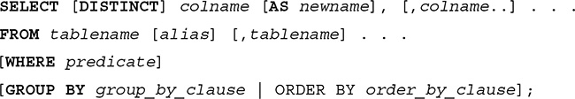
The result of executing a SELECT statement may have duplicate rows. Because duplicates are allowed, it is not a relation in the strict sense, but the result is referred to as a multiset. As indicated by the absence of square brackets, the SELECT and the FROM clauses are required, but the WHERE clause and the other clauses are optional. The rules for spacing that are common for programming languages apply to SQL, so the SELECT, FROM, and WHERE clauses can all be written on the same line if desired. Oracle includes an optional FETCH FIRST n ROWS that limits the number of rows returned to the first n. The many variations of this statement will be illustrated by the examples that follow, using the Student, Faculty, Class, and Enroll tables.
Example 1. Simple Retrieval with Condition
Query Specification: Get names, IDs, and number of credits of all Math majors.
Solution: From the Student table, we select only the rows that have a value of 'Math' for major, displaying only the lastName, firstName, stuId, and credits columns. This is the equivalent of relational algebra’s SELECT (finding the rows) and PROJECT (displaying only certain columns). We are also rearranging the columns in the result of the query.
SQL Query:

Result:

Example 2. Use of Asterisk Notation for All Columns
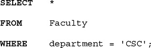
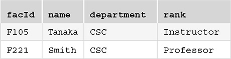
Query Specification: Get all information about CSC Faculty.
Solution: We want the entire Faculty record of any faculty member whose department is 'CSC'. Because many SQL retrievals require all columns of a single table, there is a shortcut notation, using an asterisk in place of the column names in the SELECT line.
SQL Query:
Result:
Users who access a relational database through a host language are advised to avoid using the asterisk notation. The danger is that an additional column might be added to a table after a program is written. The program will then retrieve the value of that new column with each record and will not have a matching program variable for the value, causing a loss of correspondence between database variables and program variables. It is safer to specify the columns when writing the query.
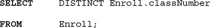
Example 3. Retrieval without Condition, Use of DISTINCT, Use of Qualified Names
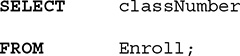
Query Specification: Get the class number of all classes in which students are enrolled.
Solution: We go to the Enroll table rather than the Class table because it is possible there is a Class record for a planned class in which no one is enrolled. From the Enroll table, we ask for all the classNumber values.
SQL Query:
Result:
classNumber ART103A CSC201A CSC201A ART103A ART103A MTH101B HST205A MTH103C MTH103C Because we did not need a predicate, we omitted the WHERE line. Notice that there are several duplicates in the result, demonstrating a result that is a multiset and not a true relation. Unlike the relational algebra PROJECT operator (π), SQL SELECT does not eliminate duplicates when it projects over columns. To eliminate the duplicates, we use the DISTINCT option after SELECT.

In any retrieval, especially if there is a possibility of confusion because the same column name appears in two different tables, we specify tablename.colname. In this example, we could have written
Here, it is not necessary to use the qualified name because the FROM line tells the system to use the Enroll table, and column names are always unique within a table. However, it is never wrong to use a qualified name, and it is sometimes necessary to do so when two or more tables appear in the FROM line.
Example 4. Retrieving an Entire Table
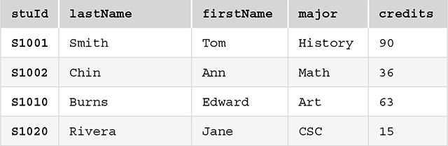
Query Specification: Get all information about all students.
Solution: Because we want all columns of the Student table, we use the asterisk notation. Because we want all the records in the table, we omit the WHERE line.
SQL Query:
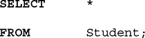
Result: The result is the entire Student table.
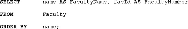
Example 5. Use of ORDER BY and AS
Query Specification: Get names and IDs of all faculty members, arranged in alphabetical order by name. Call the resulting columns FacultyName and FacultyNumber.
Solution: The ORDER BY option allows us to order the retrieved records in ascending (ASC—the default) or descending (DESC) order on any column or combination of columns, regardless of whether that column appears in the results. If we order by more than one column, the one named first determines major order, the next minor order, and so on.
SQL Query:
Result:
facultyName facultyNumber Adams F101 Byrne F110 Smith F115 Smith F221 Tanaka F105 Note the duplicate name of 'Smith'. Because we did not specify minor order, the system will arrange these two rows in any order it chooses. We could break the “tie” by giving a minor order, by changing the last line to

Note also that the column that determines ordering need not be among those displayed.
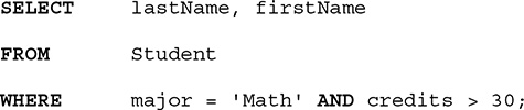
Example 6. Use of Multiple Conditions, Use of BETWEEN
Query Specification: Get names of all math majors who have more than 30 credits.
Solution: From the Student table, we choose those rows where the major is 'Math' and the number of credits is greater than 30. We express these two conditions by connecting them with AND. We display only the lastName and firstName.
SQL Query:
Result:
lastName firstName Chin Ann Jones Mary The predicate can be as complex as necessary by using the standard comparison operators =, <>, <, <=, >, and >=, and the standard logical operators AND, OR, and NOT, with parentheses, if needed or desired, to show order of evaluation.
We could modify the condition on credits using BETWEEN to specify a range of possible values. For example, to retrieve the names of math majors who are sophomores, we could have written the last line as

The BETWEEN condition here is equivalent to

5.4.2 Select Using Multiple Tables
Example 7. Natural Join
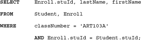
Query Specification: Find IDs and names of all students taking ART103A.
Solution: This query requires the use of two tables. We first look in the Enroll table for records where the classNumber is 'ART103A'. We then look up the Student table for records with matching stuId values and join those records into a new table. From this table, we find the lastName and firstName. This is similar to the JOIN operation in relational algebra. SQL allows us to do a natural join, as described in Section 4.5.2, by naming the tables involved and expressing in the predicate the condition that the records should match on the common column.
SQL Query:
Result:
stuId lastName firstName S1001 Smith Tom S1002 Chin Ann S1010 Burns Edward Notice that we used the qualified name for stuId in the SELECT line. We could have written Student.stuId instead of Enroll.stuId, but we needed to use one of the table names, because stuId appears in both tables in the FROM line. We did not need to use the qualified name for classNumber because it does not appear in the Student table. The fact that it appears in the Class table is irrelevant, as that table is not mentioned in the FROM line. Of course, we had to write both qualified names for stuId in the WHERE line.
Why is the condition Enroll.stuId = Student.stuId necessary? The answer is that without that condition, the result will be a Cartesian product formed by combining all Enroll records with all Student records, regardless of the values of stuId. Note that Oracle and some other RDBMSs allow the form
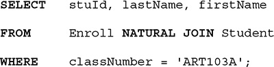
(or equivalent), which essentially adds the condition that the common columns are equal. When using the Natural Join operator qualified names are not allowed. However, because not all systems support this option, it is safest to specify the condition directly in the WHERE clause.
Example 8. Natural Join with Ordering; Use of Aliases
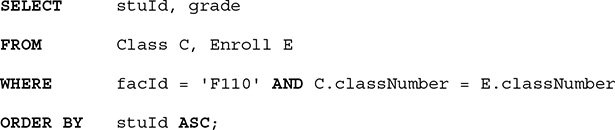
Query Specification: Find IDs and grades of all students taking any class taught by the faculty member whose faculty ID is F110. Arrange in order by student ID.
Solution: We need to look at the Class table to find the classNumber of all classes taught by F110. We then look at the Enroll table for records with matching classNumber values and get the join of the tables. From this we find the corresponding stuId and grade. Because we are using two tables, the query solution is written as a join.
In this example, we introduce aliases, which are temporary names we give to tables. We can choose any valid identifier for the alias, but it is customary to choose single letters. The alias can also be thought of as a tuple variable, a variable that ranges over all the rows of the table. An alias is introduced in the FROM line, immediately after the table name, and it replaces the table name when using qualified names for columns in the WHERE line and even in the SELECT line, if it is needed.
SQL Query:
Result:
stuId grade S1002 B S1010 S1020 A You can use the word AS between the table name and its alias, as in the following line

Example 9. Natural Join of Three Tables
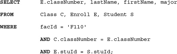
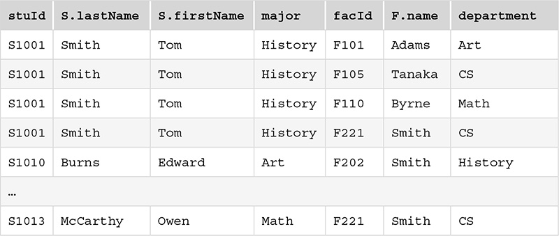
Query Specification: Find class numbers and the names and majors of all students enrolled in the classes taught by faculty member F110.
Solution: As in the previous example, we need to start at the Class table to find the classNumber of all classes taught by F110. We then compare these with classNumber values in the Enroll table to find the stuId values of all students in those classes. Then we look at the Student table to find the name and major of all the students enrolled.
SQL Query:
Result:
The query solution for Example 9 involved a natural join of three tables and required two sets of common columns. We used the condition of equality for both sets in the WHERE line. SQL ignores the order in which the tables are named in the FROM line. The same is true of the order in which we write the various conditions that make up the predicate in the WHERE line. Most sophisticated RDBMSs choose which table to use first and which condition to check first, using an optimizer to identify the most efficient method of accomplishing any retrieval before choosing a plan. This query could have been written as two natural joins

Example 10. Use of Aliases to Compare a Table to Itself
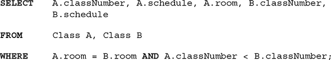
Query Specification: Get a list of all classes that meet in the same room, with their schedules and room numbers.
Solution: This query requires comparing the Class table with itself, and it would be useful if there were two copies of the table so we could do a natural join. We can pretend that there are two copies of a table by giving it two aliases, for example, A and B, and then treating these names as if they were the names of two distinct tables.
SQL Query:
Result:
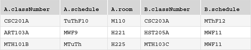
We added the second condition A.classNumber < B.classNumber to keep every class from being included because every class obviously satisfies the requirement that it meets in the same room as itself. The second condition also keeps records with the two classes reversed from appearing. For example, because we have

we do not need the record

Example 11. Theta Join
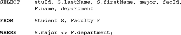
Query Specification: Find all combinations of students and faculty where the student’s major is different from the faculty member’s department.
Solution: This example illustrates a type of join in which the condition is not equality on a common column. As in relational algebra, a theta join can be done on any two tables by simply forming the Cartesian product and then applying a condition, theta. Although we usually want the natural join as in our previous examples, we might use any type of predicate as the condition for the join. If we want to compare two columns, however, they must have the same domains. In this case, the columns we are examining, major and department, do not have the same name, but they have the same domain. Because we are not told which columns to show in the result, we use our judgment.
SQL Query:
Result:
Notice that we used qualified names in the WHERE line. This was not necessary because each column name was unique, but we did so to make the condition easier to follow.
Example 12. Outer Join
Both standard SQL and Oracle support left, right, and full outer joins as described in Chapter 4, Section 4.5.2.
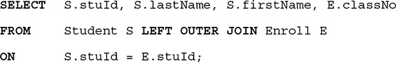
Query Specification: Find the left outer join of Student and Enroll.
SQL Query:
Result:
This will return the natural join of Student and Enroll, supplemented with those tuples of Student that do not have matches in Enroll. In place of the word LEFT in the FROM line, we can write RIGHT or FULL to find the right or full outer joins.
Example 13. Using a Subquery with Equality
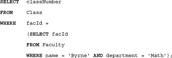
Query Specification: Find the numbers of all the classes taught by Byrne of the Math department.
Solution: We already know how to write this query using a natural join, but there is another way of finding the solution. Instead of imagining an equijoin from which we choose records with the same facId, we could visualize this as two separate queries. For the first one, we would go to the Faculty table and find the record with name of Byrne and department of Math. Then we could take the result of that query, namely F110, and search the Class table for records with that value in facId. Once we find them, we would display the classNumber. SQL allows us to sequence these queries so that the result of the first can be used in the second.
SQL Query:
Result:
classNumber MTH101B MTH103C A subquery can be used in place of a join, provided the result to be displayed is contained in a single table and the data retrieved from the subquery consists of only one column. When you write a subquery involving two tables, you name only one table in each SELECT. The query to be done first, the subquery, is the one in parentheses, following the first WHERE line. The main query is performed using the result of the subquery. Normally you want the value of some column in the table mentioned in the main query to match the value of some column from the table in the subquery. In this example, we knew we would get only one value from the subquery because facId is the key of Faculty, so a unique value would be produced. Therefore, we were able to use equality as the operator. However, conditions other than equality can be used. Any single comparison operator can be used in a subquery from which you know a single value will be produced. Because the subquery is performed first, the SELECT . . . FROM . . . WHERE of the subquery is replaced by the value retrieved, so the main query is changed to

Example 14. Subquery Using IN
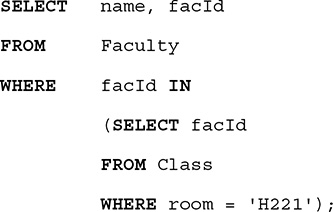
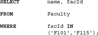
Query Specification: Find the names and IDs of all faculty members who teach a class in room H221.
Solution: We need two tables, Class and Faculty, to answer this question. We also see that the names and IDs both appear in the Faculty table, so we have a choice of a join or a subquery. If we use a subquery, we begin with the Class table to find facId values for any classes that meet in Room H221. We find two such entries from the result of the subquery. Then we go to the Faculty table and compare the facId value of each record on that table with the two facId values from Class and display the corresponding facId and name.
SQL Query:
Result:
name facId Adams F101 Smith F115 In the WHERE line of the main query we used IN, rather than =, because the result of the subquery is a set of values rather than a single value. We are saying we want the facId in Faculty to match any member of the set of values we obtain from the subquery. When the subquery is replaced by the values retrieved, the main query becomes
We can also use the negative form NOT IN, which will evaluate to true if the record has a column value that is not in the set of values retrieved by the subquery.
Example 15. Nested Subqueries
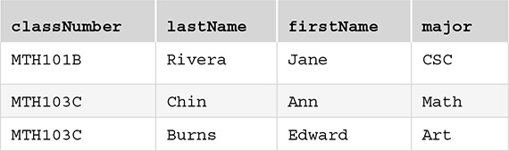
Query Specification: Get an alphabetical list of names and IDs of all students in any class taught by F110.
Solution: We need three tables, Student, Enroll, and Class, to answer this question. However, the values to be displayed appear in one table, Student, so we can use a subquery. First, we check the Class table to find the classNumber of all classes taught by F110. We find two values, MTH101B and MTH103C. Next, we go to the Enroll table to find the stuId of all students in either of these classes. We find three values, S1020, S1010, and S1002. We now look at the Student table to find the records with matching stuId values, and display the stuId, lastName, and firstName in alphabetical order by name.
SQL Query:
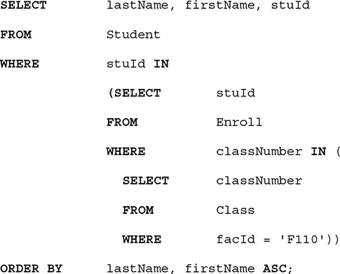
Result:
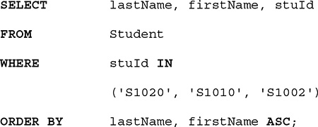
lastName firstName stuId Burns Edward S1010 Chin Ann S1002 Rivera Jane S1020 In execution, the most deeply nested SELECT is done first, and it is replaced by the values retrieved, so we have
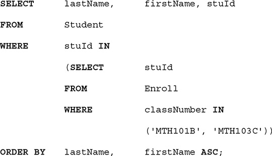
Next the subquery on Enroll is done, and we get
Finally, the main query is done, and we get the result shown earlier. Note that the ordering refers to the final result, not to any intermediate steps, and it appears at the end. Also note that we could have performed either part of the operation as a natural join and the other part as a subquery, mixing both methods.
Example 16. Query Using EXISTS or NOT EXISTS
Example 16(a). Query Using EXISTS
Query Specification: Find all students enrolled in any class.
Solution: We already know how to write this query using a join or a subquery with IN. However, another way of expressing this query is to use the existential quantifier, EXISTS, with a subquery.
SQL Query:
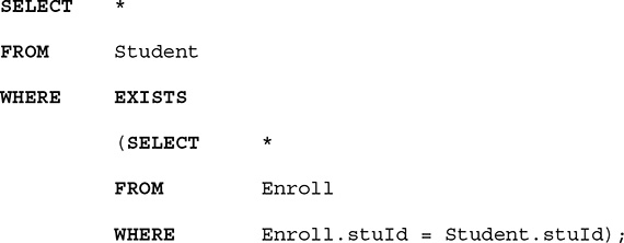
Result:
This query could be phrased as “Find the names of all students such that there exists an enrollment record containing their student Id.” It is identical to the relational algebra semijoin (⋉ or ⋊) (as described in Chapter 4). The test for inclusion is the existence of such a record. If it exists, the EXISTS (SELECT FROM . . .) evaluates to true. Notice we needed to use the name of the main query table, Student, in the subquery to express the condition Student.stuId = Enroll.stuId. In general, we avoid mentioning a table not listed in the FROM for that particular query, but it is necessary and permissible to do so in this case. This form is called a correlated subquery because the table in the subquery is being compared to the table in the main query.
Example 16(b). Query Using NOT EXISTS
Query Specification: Find the names of all students who are not enrolled in any class.
Solution: We could rephrase this query as “Select names of students from the Student table such that no Enroll record exists that contains their stuId values.” Unlike the previous example, we cannot readily express this query using a join or an IN subquery. Instead, we will use NOT EXISTS. This operation is sometimes called the antijoin because it returns records that do not participate in the join.
SQL Query:
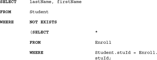
Result:
lastName firstName Lee Perry McCarthy Owen Jones Mary Example 17. Query Using NULL
Query Specification: Find the student name and class number of all students whose grades in that class are missing.
Solution: This query involves a missing value in a column, not a missing record, so we cannot use NOT EXISTS as in the previous example. We can see from the Enroll table that there are two Enroll records with missing grades. You might think they could be accessed by specifying that the grades are not A, B, C, D, or F, but that is not the case. A null grade is considered to have “unknown” as a value, so it is impossible to judge whether it is equal to or not equal to another grade. If we put the condition WHERE grade <>'A' AND grade <>'B' AND grade <>'C' AND grade <>'D' AND grade <>'F', we would get an empty table back instead of the two records we want. SQL uses the logical expression

to test for null values in a column.
SQL Query:
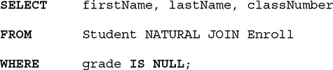
Result:
firstName lastName classNumber Edward Burns ART103A Edward Burns MTH103C Notice that it is incorrect to write WHERE grade = NULL because a predicate involving comparison operators with NULL will evaluate to “unknown” rather than “true” or “false.” The WHERE line is the only one on which NULL can appear in a SELECT statement.
Example 18. Queries Using Set Operators
Query Specification: Get IDs of all faculty who are assigned to the History department or who teach in room H221.
Solution: We could use the natural join and an OR operator to express this query as
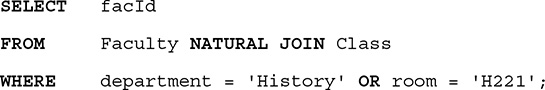
As an alternative approach, we will do a simple selection on each table, returning just the facId from each. Because the results sets have the same structure, they are union compatible. We can combine the results from the two queries by using a UNION operator. UNION in SQL is the standard relational algebra operator for set union, and it works in the expected way, eliminating duplicates.
SQL Query:
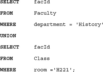
Result:
facId F101 F115 In addition to UNION, SQL supports the operations INTERSECT and MINUS, which perform the standard set operations of set intersection and set difference on union compatible tables, and UNION ALL, INTERSECT ALL, and MINUS, which operate like their counterparts, except that they do not eliminate duplicate rows.
5.4.3 Select with Aggregate Functions
SQL has a large number of built-in functions, including aggregate functions. These functions operate on a single column of a table. The most commonly used SQL aggregate functions are COUNT, SUM, AVG, MIN, and MAX. Oracle also includes VARIANCE and STDDEV. In addition, Oracle has more sophisticated statistical and analytical aggregate functions. These functions will be discussed in Chapter 12.
| Function | Return |
|---|---|
| COUNT | Returns the number of values in the column |
| SUM | Returns the sum of the values in a numeric column |
| AVG | Returns the mean of the values in a numeric column |
| MAX | Returns the largest value in the column |
| MIN | Returns the smallest value in the column |
| VARIANCE | Returns the variance of values in a numeric column |
| STDDEV | Returns the standard deviation of values in a numeric column |
Normally, aggregate functions eliminate rows with null values in the column first and then perform the operation on the remaining rows, returning a single result for those rows. If the column can have duplicate values, the keyword DISTINCT (or UNIQUE) can be used to eliminate duplicates first, or the keyword ALL can be used to keep the duplicates before the computation is done. If neither is specified, the default is ALL. If we use DISTINCT with MAX or MIN it will have no effect because the largest or smallest value remains the same even if two tuples share it. However, DISTINCT usually has an effect on the result of SUM, AVG, VARIANCE, and STDDEV, so the user should understand whether or not duplicates should be included in computing these.
Example 19. Using COUNT and COUNT(*)
Query Specification: Find the total number of students enrolled in classes.
Solution: For this query, we will use COUNT, which returns the number of non-null values in a column. We want to eliminate duplicates because a student may be enrolled in several classes, so we use DISTINCT.
SQL Query:
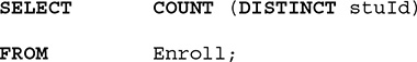
The result is 4. If we had written the query without the keyword DISTINCT, the result would have been 9.
COUNT(*) is a special use of COUNT. Its purpose is to count all the rows of a table, regardless of whether null values or duplicate values occur. If we write
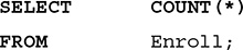
The result of the query is 9.
Example 20. Using SUM
Query Specification: Find the sum of all the credits that history majors have.
Solution: We want to include all students who are history majors, so we do not use DISTINCT here, or else two history majors with the same number of credits would be counted only once.
SQL Query:
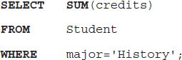
The result is 93
Example 21. Using AVG
Query Specification: Find the average number of credits students have.
Solution: We do not want to use DISTINCT in this query because if two students have the same number of credits, both should be counted in the average.
SQL Query:
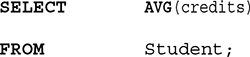
The result is 35.5714286.
Example 22. Using MAX
Query Specification: Find the student with the largest number of credits.
Solution: Because we want the student’s credits to equal the maximum, we need to find that maximum first, so we use a subquery to find it, then find the student with that number of credits. If more than one student qualifies, all the ties will be returned.
SQL Query:
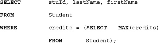
Result:
stuId lastName firstName S1001 Smith Tom It may be tempting to put the function in the SELECT phrase along with the student information, as in

but that approach to writing the query will not work, producing an error message saying that MAX is not a single-group group function. The SELECT line is mixing information about individual rows with a function that applies to the whole group, which is not allowed.
Example 23. Using MIN
Query Specification: Find the ID of the student(s) with the highest grade in any course.
Solution: Because we want the highest grade, it might appear that we should use the MAX function here. A closer look at the table reveals that the grades are letters A, B, C, etc. For this scale, the best grade is the one that is earliest in the alphabet, so we actually want to use the MIN function. If the grades were numeric, we would have used the MAX function The collating sequence is used to determine order of non-numeric data.
SQL Query:
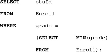
The result is S1001 and S1020.
Example 24. Using AVG
Query Specification: Find names and IDs of students who have less than the average number of credits.
Solution: We first must find the average number of credits in a subquery, and then find the students who have fewer credits.
SQL Query:
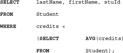
The result is the ID values and names of students S1005, S1013, and S1020.
Example 25. Using VARIANCE
In statistics, the variance of a set of numbers is a measure of how spread out the numbers are from the mean of the set. It is the average of the squares of the difference of each of the values from the mean. The larger this value, the more spread out the numbers are.
Query Specification: Find the variance of the credits values.
SQL Query:

The result is 1084.28571.
Example 26. Using STDDEV
Standard deviation is also used to measure spread from the mean. It is defined to be the square root of the variance.
Query Specification: Find the standard deviation of the credits values.
SQL Query:
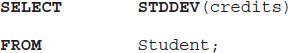
The result is 32.928494
Example 27. Using an Expression and a String Constant; Using the Concatenation Operator || Query Specification: Assuming each course is three credits, list, for each student, the number of courses completed.
Solution: We can use the expression credits/3 in the SELECT to display the number of courses. Because we have no such column name, we will use a string constant as a label. String constants that appear in the SELECT line are simply printed on each line in the result.
SQL Query:
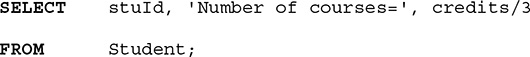
Result:
stuId 'Numberofcourses=' credits/3 S1001 Number of courses = 30 S1010 Number of courses = 21 S1015 Number of courses = 14 S1005 Number of courses = 1 S1002 Number of courses = 12 S1020 Number of courses = 5 S1013 Number of courses = 0 To eliminate the space between the string constant and the number of courses, we can use the concatenation operator for strings, ||
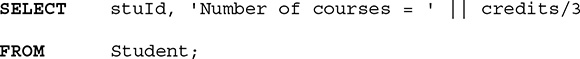
By combining constants, column names, arithmetic operators, built-in functions, and parentheses, the user can customize retrievals.
Example 28. Adding ORDER BY with a Row Limit
Query Specification: For the same query as in Example 27, order students by number of courses and limit the rows to 50% but include ties if two students have the same number of courses.
Solution: Add FETCH FIRST ... ROWS option.
SQL Query:

Result:
stuId 'Numberofcourses=' || credits/3 S1013 Number of courses = 0 S1005 Number of courses = 1 S1020 Number of courses = 5 S1002 Number of courses = 12 Instead of specifying a percent, you can specify the number of rows to be returned as in

Example 29. Using a Row Limit with Offset
Query Specification: For the same query as in Example 27, order students by number of classes and limit the returned rows to 2, but do not include the first two records and do not include ties.
Solution: When using the ORDER BY clause, we can choose to specify a number or percentage of rows to be skipped using the OFFSET option

SQL Query:
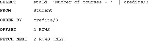
The result is just the last two rows of the previous result.
5.4.4 SELECT with GROUP BY
The GROUP BY clause allows us to put together all the records with a single value in the specified column. Then we can apply any aggregate function to any column in each group, provided the result is a single value for the group.
Example 30. Using GROUP BY with SUM
Query Specification: For each major, find the sum of all the credits that the students with that major have.
Solution: We want to use the SUM function, but we need to apply it to each major individually. We use GROUP BY to group the Student records by majors and use the SUM function on the credits column in each group to obtain the result. Note that this time the function appears in the SELECT line because it applies to a group, not to single records.
SQL Query:
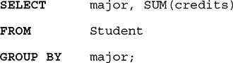
Result:
major SUM(credits) History 93 Math 78 Art 63 CSC 15 Example 31. Using GROUP BY with COUNT(*)
Query Specifications: For each class, show the number of students enrolled.
Solution: We want to use the COUNT function, but we need to apply it to each class individually. We use GROUP BY to group the records into classes, and we use the COUNT function on each group to obtain the result.
SQL Query:
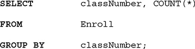
Result:
classNumber COUNT(*) ART103A 3 CSC201A 2 MTH101B 1 HST205A 1 MTH103C 2 Note that we could have used COUNT(DISTINCT stuId) in place of COUNT(*) in this query.
Example 32. Using GROUP BY ... HAVING
GROUP BY ... HAVING is used to determine which groups have some quality, just as WHERE is used with tuples to determine which records have some quality. You are not permitted to use HAVING without GROUP BY, and the predicate in the HAVING line must have a single value for each group.
Query Specification: Find all courses in which fewer than three students are enrolled.
Solution: This is a question about a characteristic of the groups formed in the previous example. We use HAVING COUNT(*) as a condition on the groups.
SQL Query:
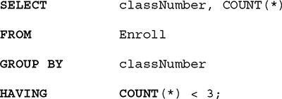
Result:
classNumber COUNT(*) CSC201A 2 HST205A 1 MTH101B 1 MTH103C 2 Example 33. Using GROUP BY ... HAVING with a Subquery
Query Specification: Find all major departments where the average of students’ credits is less than the average number of credits all students have.
Solution: We use a subquery to find the average number of credits all students have. In the main query we group the students by major department, calculate the average credits for each group, and ask for those whose average is below the total average.
SQL Query:
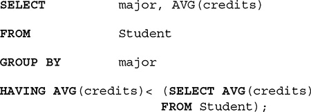
Result:
major AVG(credits) Math 26 CSC 15
5.4.5 SELECT with Pattern Strings
SQL allows us to use LIKE in a predicate to display a pattern string for character columns. Records whose specified columns match the pattern will be retrieved. In the pattern string, we can use the symbols %, _, and other characters as shown in the following table.
| character | use in pattern string |
|---|---|
| % | Any sequence of characters of any length >= 0 |
| _ (underscore) | Any single character |
| a...z. A..Z, 0..9, etc. (any single character) | All other characters stand for themselves |
Examples:
classNumber LIKE 'MTH% ' means the first three letters must be MTH, but the rest of the string can be any characters.
stuId LIKE 'S_ _ _ _' means there must be five characters, the first of which must be an S.
schedule LIKE '%9' means any sequence of characters, of length at least one, with the last character a 9.
classNumber LIKE '%101%' means a sequence of characters of any length containing 101. Note the 101 could be the first, last, or only characters, as well as being somewhere in the middle of the string.
name NOT LIKE 'A%' means the name cannot begin with an A.
Example 34. Using LIKE
Query Specification: Get details of all math courses.
Solution: We want the first three letters of classNumber to be MTH.
SQL Query:

Result:

Example 35. Using REGEXP_LIKE
In addition to LIKE and NOT LIKE, Oracle supports the use of REGEXP_LIKE, which compares the value of an attribute to a regular expression. Regular expressions are a way of expressing complex pattern strings, and are used in Java, Python, and PERL. They contain literals, which are the characters to be searched for, and metacharacters, which are operators that specify what search algorithms are to be used.
The form is
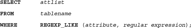
The REGEXP_LIKE operator is called RLIKE in some versions of SQL.
Query Specification: Find all faculty whose names are either Smith or Smyth.
SQL Query:
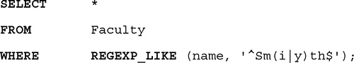
Result:
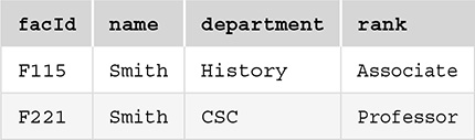
The regular expression '^Sm(i|y)th$' specifies a string that begins with Sm, immediately followed by either i or y, immediately followed by th, which is the end of the string.
5.4.6 Operators for Updating: UPDATE, INSERT, DELETE
UPDATE
The UPDATE operator is used to change values in records already stored in a table. UPDATE is used on one table at a time, and can change zero, one, or many records, depending on the predicate. Its form is

Note that it is not necessary to specify the current value of the column, although the present value may be used in the expression to determine the new value. Note that you cannot update a column that has been created as an IDENTITY column in Oracle.
Example 1. Updating a Single Column of One Record
Operation: Change the major of S1020 to Music.
SQL Command:

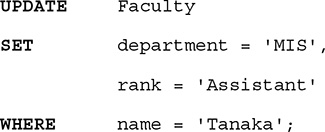
Example 2. Updating Several Columns of One Record
Operation: Change Tanaka’s department to MIS and rank to Assistant.
SQL Command:
Example 3. Updating Using NULL
Operation: Change the major of S1013 from Math to NULL.
To insert a null value into a column that already has an actual value, we must use the form

SQL Command:

Example 4. Updating Several Records
Operation: Change grades of all students in CSC201A to A.
SQL Command:

Example 5. Updating All Records
Operation: Give all students three extra credits.
SQL Command:
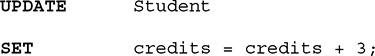
Notice we did not need the WHERE line because all records were to be updated.
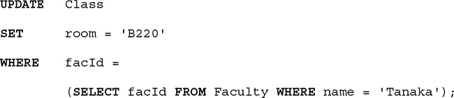
Example 6. Updating with a Subquery
Operation: Change the room to B220 for all classes taught by Tanaka.
SQL Command:
INSERT
The INSERT operator is used to put new records into a table. Normally, it is not used to load an entire table because the DBMS usually has a load utility to handle that task. However, the INSERT is useful for adding one or a few records to a table. The form of the INSERT operator is:
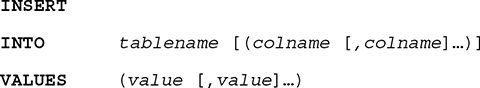
The column names are optional if we are inserting values for all columns in their proper order. We can also write DEFAULT in place of an actual value, provided the column has a default specified.
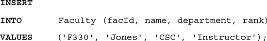
Example 1. Inserting a Single Record with All Columns Specified
Operation: Insert a new Faculty record with ID of F330, name of Jones, department of CSC, and rank of Instructor.
SQL Command:
Example 2. Inserting a Single Record without Specifying Columns
Operation: Insert a new student record with ID of S1030, name of Alice Hunt, major of Art, and 12 credits.
SQL Command:
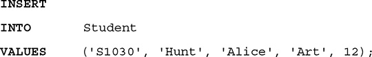
Here, it was not necessary to specify column names because the system assumes that we are inserting all the columns in the table in their correct order. We could have done the same for the previous example.
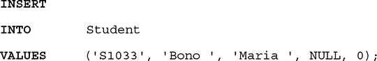
Example 3. Inserting a Record with Null Value in a Column
Operation: Insert a new student record with ID of S1031, name of Maria Bono, zero credits, and no major.
SQL Command:

Although we rearranged the column names, there is no confusion because it is understood that the order of values matches the order of columns named in the INTO line, regardless of their order in the table. Also notice the zero is an actual value for credits, not a null value. The major value will be set to null because we excluded it from the column list in the INTO line, unless we had specified a default value for it when we created the table.
Another method for setting a value to null is to use the value NULL in the place occupied by the missing column. For example, we could have written
Example 4. Inserting Multiple Records into a New Table
Operation: Create and fill a new table that shows each class and the number of students enrolled in it.
SQL Command:
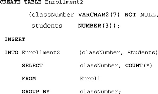
Here, we created a new table, Enrollment2, and filled it by taking data from an existing table, Enroll. Enrollment2 looks like this:
Enrollment2 classNumber Students ART103A 3 CSC201A 2 MTH101B 1 HST205A 1 MTH103C 2 The Enrollment2 table is now available for the user to manipulate, just as any other table would be. It can be updated as needed, but it will not be updated automatically when the Enroll table is updated.
Example 5. Inserting Values Using a Query
A query can be embedded in an INSERT or UPDATE statement to determine a value for a column in a record.
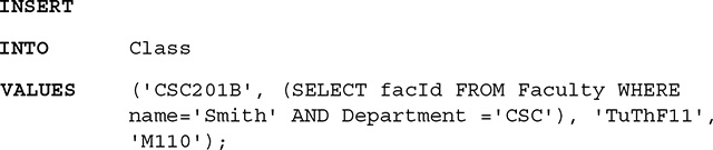
Operation: Insert a new class record for CSC201B, to be taught by Smith of the CSC department. The class meets on Tuesday, Thursday, and Friday at 11 in room M110.
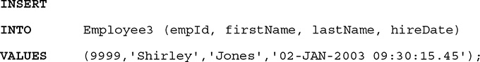
Example 6. Inserting DATE and TIMESTAMP Values
For the following examples, use the schema

which is created using the DDL command

Example 6(a). Inserting a DATE Value Using Default Format
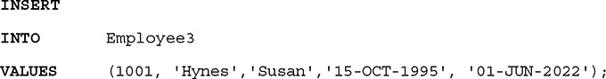
The simplest way to insert dates in Oracle is to use the default format 'DD-MON-YY', as in '01-JAN-22'.
Operation: Insert a new employee record for Susan Hynes, born Oct 15, 1995, hired on June 1, 2022.
SQL Command:
Example 6(b). Inserting a Record Using SYSDATE
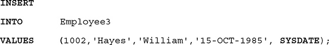
Operation: Insert a new record for William Hayes, born Oct 15, 1985, hired today, using SYSDATE. To set the hireDate value to the date the record is inserted, we use SYSDATE, which returns the current system date and time, accurate to the second.
SQL Command:
Example 6(c). Changing a Data Type from DATE to TIMESTAMP
A TIMESTAMP column can store date and time accurately to fractions of a second. Although this precision is not needed for most records, it becomes important when we are tracking transactions and we need to know to a fraction of a second when a transaction started and ended.
Operation: Convert the hireDate column of the Employee3 table to the TIMESTAMP type.
SQL Command:

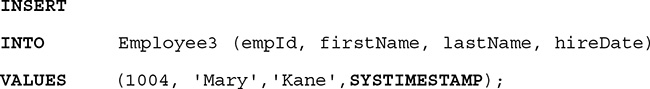
Example 6(d). Entering Data for a TIMESTAMP Column Using SYSTIMESTAMP
Operation: Enter a new employee record using SYSTIMESTAMP, which is the current system timestamp, for the hireDate column.
SQL Command:
Example 6(e). Entering Data for a TIMESTAMP Column Using Oracle Default Format
Oracle uses the default format 'DD-MON-YY HH:MI:SS.FF' for timestamp values, as shown in the following example.
SQL Command:
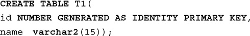
Example 7. Creating and Using IDENTITY Columns
As explained in Section 5.2, Oracle supports identity columns and generates values for them. In the CREATE TABLE command, the line

creates a column called id that is populated automatically by Oracle. The user can change the starting value and the increment by adding

Example 7(a). Creating a Table with an Always IDENTITY Column
The default type of IDENTITY column is called an always IDENTITY column because the system, and never the user, supplies the value.
Operation: Create a table with an always IDENTITY column and a name. Make the identity column the primary key.
SQL Command:
Example 7(b). Inserting Records Containing an Always IDENTITY Column
Operation: Insert two records into a table T1, which has an always IDENTITY column, and view the results.
SQL Command:
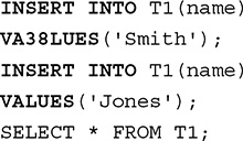
Result:
id name 1 Smith 2 Jones We never supply a value for an always IDENTITY column, but instead specify the other columns of the table for which values are supplied. The system keeps track of the values it generates for the IDENTITY column for each table that has one. Unless the user specifies a different starting value and increment, it will begin with 1 and will increment the value of the column by 1 each time a new record is created, even if old records have been deleted, and even if the user session has ended and a new one has begun.
Example 7(c). Creating a Default-Only IDENTITY Column
It is also possible to specify that the IDENTITY value is system-generated only when the user fails to provide a value for the column, called a default only IDENTITY column. This will allow the user to input id values, but for any record lacking a value, the system will create a unique id by default.
Operation: Create a table with a default-only IDENTITY column and a color. Start the default values at 100 and increment by 10.
SQL Command:

Example 7(d). Inserting Records into a Default-Only IDENTITY Column
Operation: Insert a record, giving a value for the id column. Insert a second record without giving a value for the id column. View both records.
SQL Command:
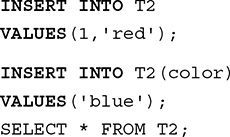
Result:
id color 1 red 100 blue
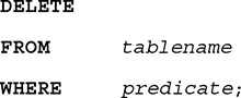
DELETE
The DELETE command is used to erase records. The number of records deleted may be zero, one, or many, depending on how many satisfy the predicate. The form of this command is
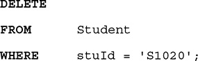
Example 1. Deleting a Single Record
Operation: Erase the record of student S1020.
SQL Command:
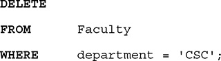
Example 2. Deleting Several Records
Operation: Erase all faculty records where the department is CSC.
SQL Command:
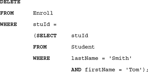
Example 3. DELETE with a Subquery
Operation: Erase all enrollment records for Tom Smith.
SQL Command:
Example 4. Deleting All Records from a Table
Operation: Erase all the class records.
If we deleted Class records and allowed their corresponding Enroll records to remain, we would lose referential integrity because the Enroll records would then refer to classes that no longer exist. However, when we created the tables using Oracle and the commands shown in Figure 5.2, we wrote

for the Enroll table. Therefore, when we delete Class records, their corresponding Enroll records will be deleted as well because we chose CASCADE.
SQL Command:

This removes all records from the Class table and the Enroll table, but their structure remains, so we could add new records to them at any time.