
Chapter 5
Hearing Timbre and Deceiving the Ear
Chapter Contents
- 5.1 What Is Timbre?
- 5.2 Acoustics of Timbre
- 5.3 Psychoacoustics of Timbre
- 5.4 The Pipe Organ as a Timbral Synthesizer
- 5.5 Deceiving the Ear
- References
5.1 What Is Timbre?
Pitch and loudness are two of three important descriptors of musical sounds commonly used by musicians, the other being “timbre.” Pitch relates to issues such as notes on a score, key, melody, harmony, tuning systems and intonation in performance. Loudness relates to matters such as musical dynamics (e.g., pp, p, mp, mf, f, ff) and the balance between members of a musical ensemble (e.g., between individual parts, choir and orchestra or soloist and accompaniment). Timbre-to-sound quality descriptions include: mellow, rich, covered, open, dull, bright, dark, strident, grating, harsh, shrill, sonorous, somber, colorless and lackluster. Timbral descriptors are therefore used to indicate the perceived quality or tonal nature of a sound that can have a particular pitch and loudness also.
There is no subjective rating scale against which timbre judgments can be made, unlike pitch and loudness which can, on average, be reliably rated by listeners on scales from “high” to “low.” The commonly quoted American National Standards Institute formal definition of timbre reflects this: “Timbre is that attribute of auditory sensation in terms of which a listener can judge two sounds similarly presented and having the same loudness and pitch as being dissimilar” (ANSI, 1960). In other words, two sounds that are perceived as being different but that have the same perceived loudness and pitch differ by virtue of their timbre (consider the examples on track 62 of the accompanying CD). The timbre of a note is the aspect by which a listener recognizes the instrument that is playing a note when, for example, instruments play notes with the same pitch, loudness and duration.
The definition given by Scholes (1970) encompasses some timbral descriptors: “Timbre means tone quality—coarse or smooth, ringing or more subtly penetrating, ‘scarlet’ like that of a trumpet, ‘rich brown’ like that of a cello, or ‘silver’ like that of the flute. These color analogies come naturally to every mind…. The one and only factor in sound production which conditions timbre is the presence or absence, or relative strength or weakness, of overtones.” (In Chapter 3, Table 3.1 gives the relationship between overtones and harmonics.) While his color analogies might not come naturally to every mind, Scholes’s later comments about the acoustic nature of sounds which have different timbres are a useful contribution to the acoustic discussion of the timbre of musical sounds.
When considering the notes played on pitched musical instruments, timbre relates to those aspects of the note that can be varied without affecting the pitch, duration or loudness of the note as a whole, such as the spectral components present and the way in which their frequencies and amplitudes vary during the sound. In Chapter 4, the acoustics of musical instruments are considered in terms of the output from the instrument as a consequence of the effect of the sound modifiers on the sound input (e.g., Figure 4.2). What is not considered, due to the complexity of modeling, is the acoustic development from silence at the start of the note and back to silence at the end. It is then convenient to consider a note in terms of three phases: the “onset” or “attack” (the buildup from silence at the start of the note), the “steady state” (the main portion of the note) and the “offset” or “release” (the return to silence at the end of the note after the energy source is stopped). The onset and offset portions of a note tend to last for a short time, on the order of a few tens of milliseconds (or a few hundredths of a second). Changes that occur during the onset and offset phases, and in particular during the onset, turn out to have a very important role in defining the timbre of a note.
In this chapter, timbre is considered in terms of the acoustics of sounds that have different timbres and the psychoacoustics of how sounds are perceived. Finally, the pipe organ is reviewed in terms of its capacity to synthesize different timbres.
5.2 Acoustics of Timbre
The description of the acoustics of notes played on musical instruments presented in Chapter 4 was in many cases supported by plots of waveforms and spectra of the outputs from some instruments (Figures 4.17, 4.22, 4.24 and 4.29). Except in the plots for the plucked notes on the lute and guitar (Figure 4.11), where the waveforms are for the whole note and the spectra are for a single spectral analysis, the waveform plots show a few cycles from the steady-state phase of the note concerned, and the spectral plots are based on averaging together individual spectral measurements taken during the steady-state phase. The number of spectra averaged together depends on how long the steady-state portion of the note lasts. For the single notes illustrated in Chapter 4, spectral averaging was carried out over approximately a quarter to three quarters of a second, depending on the length of the note available.
An alternative way of thinking about this is in terms of the number of cycles of the waveform over which the averaging takes place, which would be 110 cycles for a quarter of a second to 330 cycles for three quarters of a second for A4 (f0 = 440 Hz), or 66 cycles to 198 cycles for C4 (f0 = 261.6 Hz). Such average spectra are commonly used for analyzing the frequency components of musical notes, and they are known as “long-term average spectra” or “LTAS.” One main advantage of using LTAS is that the spectral features of interest during the steady-state portion of the note are enhanced in the resulting plot by the averaging process with respect to competing acoustic sounds, such as background noise, which change over the period of the LTAS and thus average toward zero.
LTAS cannot, however, be used to investigate acoustic features that change rapidly such as the onset and offset of musical notes, because these will also tend to average toward zero. In terms of the timbre of the note, it is not only the variations that occur during the onset and offset that are of interest but also how they change with time. Therefore an analysis method is required in which the timing of acoustic changes during a note is preserved in the result. One analysis technique commonly used for the acoustic analysis of speech is a plot of amplitude, frequency and time known as a “spectrogram.” Frequency is plotted on the vertical scale; time on the horizontal axis and amplitude is plotted as the darkness on a gray scale, or in some cases the color, of the spectrogram.
The upper plot in Figure 5.1 shows a spectrogram and acoustic pressure waveform of C4 played on a principal 8′ (open flue), the same note for which an LTAS is presented in Figure 4.17. The LTAS plot in Figure 4.17 showed that the first and second harmonics dominate the spectrum, the amplitude of the third harmonic being approximately 8 dB lower than the first harmonic, and with energy also clearly visible in the fourth, fifth, seventh and eighth harmonics, whose amplitudes are at least 25 dB lower than that of the first harmonic.
A spectrogram shows which frequency components are present (measured against the vertical axis), at what amplitude (blackness of marking) and when (measured against the horizontal axis). Thus harmonics are represented on spectrograms as horizontal lines, where the vertical position of the line marks the frequency and the horizontal position shows the time for which that harmonic lasts. The amplitudes of the harmonics are plotted as the blackness of marking of the lines. The frequency and time axes on the spectrogram are marked, and the amplitude is shown as the blackness of the marking.
The spectrogram shown in Figure 5.1 shows three black horizontal lines, which are the first three harmonics of the principal note (since the frequency axis is linear, they are equally spaced). The first and second harmonics are slightly blacker (and thicker) than the third, reflecting the amplitude difference as shown in Figure 4.17. The fourth, fifth and seventh harmonics are visible, and their amplitude relative to the first harmonic is reflected in the blackness with which they are plotted.
5.2.1 Note Envelope
The onset, steady-state, and offset phases of the note are indicated above the waveform in the figure, and these are determined mainly with reference to the spectrogram because they relate to the changes in spectral content at the start and end of the note, leaving the steady portion in between. However, “steady state” does not mean that no aspect of the note varies. The timbre of a principal organ stop sounds “steady” during a prolonged note such as that plotted, which lasts for approximately 2 seconds, but it is clear from the acoustic pressure waveform plot in Figure 5.1 that the amplitude, or “envelope,” varies even during the so-called steady-state portion of this note. This is an important aspect of musical notes to be aware of when, for example, synthesizing notes of musical instruments, particularly if using looping techniques on a sampling synthesizer.
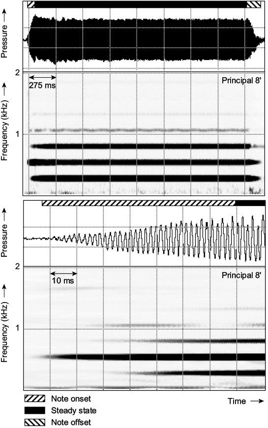
For the principal pipe, the end of the note begins when the key is released and the air flowing from the organ bellows to drive the air reed is stopped. In the note offset for this example, which lasts approximately 200 ms, the high harmonics die away well before the first and second. However, interpretation of note offsets is rather difficult if the recording has been made in an enclosed environment as opposed to free space (see Chapter 4), since any reverberation due to the acoustics of the space is also being analyzed (see Chapter 6). It is difficult to see the details of the note onset in this example due to the timescale required to view the complete note.
The note onset phase is particularly important to perceived timbre. Since listeners can reliably perceive the timbre of notes during the steady-state phase, it is clear that the offset phase is rather less important to the perception of timbre than the onset and steady-state phases. The onset phase is also more acoustically robust from the effects of the local environment in which the notes are played, since coloration of the direct sound by the first reflection (see Chapter 6) may occur after the onset phase is complete (and therefore transmitted uncolored to the listener). By definition, the first reflection certainly occurs after part of the note onset has been heard uncolored. The onset phase is therefore a vital element and the offset phase an important factor in terms of timbre perception. Spectrograms whose timescales are expanded to cover the time of the note onset phase are particularly useful when analyzing notes acoustically.
The lower plot in Figure 5.1 shows an expanded timescale version of the upper plot in the figure, showing the note onset phase, which lasts approximately 70 ms, and the start of the steady-state phase. It can be seen that the detail of the onset instant of each of the harmonics is clearly visible, with the second harmonic starting approximately 30 ms before the first and third harmonics. This is a common feature of organ pipes voiced with a chiff or consonantal onset, which manifests itself acoustically in the onset phase as an initial jump to the first, or sometimes higher, overblown mode.
The first overblown mode for an open flue pipe is to the second harmonic (see Chapter 4). Careful listening to pipes voiced with a chiff will reveal that open pipes start briefly an octave high since their first overblown mode is the second harmonic, and stopped pipes start an octave and a fifth high since their first overblown mode is the third harmonic. The fourth harmonic in the figure starts with the third, and its amplitude briefly drops 60 ms into the sound when the fifth starts, and the seventh starts almost with the second, and its amplitude drops 30 ms later. The effect of the harmonic buildup on the acoustic pressure waveform can be observed in Figure 5.1 in terms of the changes in its shape, particularly the gradual increase in amplitude during the onset phase. The onset phase for this principal organ pipe is a complex series of acoustic events, or acoustic “cues,” which are available as potential contributors to the listener’s perception of the timbre of the note.
5.2.2 Note Onset
In order to provide some data to enable appreciation of the importance of the note onset phase for timbre perception, Figures 5.2 to 5.4 are presented, in which the note onset and start of the steady-state phases for four organ stops, four woodwind instruments and four brass instruments, respectively, are presented for the note C4 (except for the trombone and tuba, for which the note is C3). By way of a caveat, it should be noted that these figures are presented to provide only examples of the general nature of the acoustics of the note onset phases for these instruments. Had these notes been played at a different loudness, by a different player, on a different instrument, in a different environment or even just a second time by the same player on the same instrument in the same place while attempting to keep all details constant, the waveforms and spectra would probably be noticeably different.
The organ stops for which waveforms and spectra are illustrated in Figure 5.2 are three reed stops: hautbois and trompette (LTAS in Figure 4.22) and a regal, and gedackt (LTAS in Figure 4.17), which is an example of a stopped flue pipe. The stopped flue supports only the odd modes (see Chapter 4), and, during the onset phase of this particular example, the fifth harmonic sounds first, which is the second overblown mode sounding two octaves and a major third above the fundamental (see Figure 3.3), followed by the fundamental and then the third harmonic, giving a characteristic chiff to the stop.
The onset phase for the reed stops is considerably more complicated since many more harmonics are present in each case. The fundamental for the hautbois and regal is evident first, and the second harmonic for the trompette. In all cases, the fundamental exhibits a frequency rise at onset during the first few cycles of reed vibration. The staggered times of entry of the higher harmonics form part of the acoustic timbral characteristic of that particular stop, the trompette having all harmonics present up to the 4 kHz upper frequency bound of the plot, the hautbois having all harmonics up to about 2.5 kHz, and the regal exhibiting little or no evidence (at this amplitude setting of the plot) of the fourth or eighth harmonics.
Figure 5.3 shows plots for four woodwind instruments: clarinet, oboe, tenor saxophone and flute. For these particular examples of the clarinet and tenor saxophone, the fundamental is apparent first, and the oboe note begins with the second harmonic, followed by the third and fourth harmonics after approximately 5 ms, and then the fundamental some 8 ms later. The higher harmonics of the clarinet are apparent nearly 30 ms after the fundamental; the dominance of the odd harmonics is discussed in Chapter 4.
This particular example of C4 from the flute begins with a notably “breathy” onset just prior to and as the fundamental component starts. This can be seen in the frequency region of the spectrogram that is above 2 kHz lasting some 70 ms. The higher harmonics enter one by one approximately 80 ms after the fundamental starts. The rather long note onset phase is characteristic of a flute note played with some deliberation. The periodicity in the waveforms develops gradually, and in all cases there is an appreciable time over which the amplitude of the waveform reaches its steady state.

Figure 5.4 shows plots for four brass instruments. The notes played on the trumpet and French horn are C4, and those for the trombone and tuba are C3. The trumpet is the only example with energy in high harmonic components in this particular example, with the fourth, fifth and sixth harmonics having the highest amplitudes. The other instruments in this figure do not have energy apparent above approximately the fourth harmonic (French horn and tuba) or the sixth harmonic for the trombone. The note onset phase for all four instruments starts with the fundamental (noting that this is rather weak for the trombone), followed by the other harmonics. The waveforms in all cases become periodic almost immediately.

5.2.3 Steady State
The steady-state portion of a note is important to the perception of the timbre of a note. It has been pointed out that even for a note on an instrument such as the pipe organ, where one might expect the note to be essentially fixed in amplitude during the steady-state part (see Figure 5.1), there is considerable variation. For some musical instruments, such as those in the orchestral string section (violin, viola, cello, double bass), the human voice (particularly in opera solo singing) and to some extent the woodwinds (oboe, clarinet, saxophone, bassoon), an undulation during the steady-state part of the notes is manifest naturally in the acoustic output. This is usually in the form of vibrato and/or tremolo. Vibrato is a variation in fundamental frequency, or frequency modulation, and tremolo is a variation in amplitude, or amplitude modulation.

Waveforms and spectrograms are presented in the upper plot of Figure 5.5 for C4 played with a bow on a violin. Approximately 250 ms into the violin note, vibrato is apparent as a frequency variation, particularly in the high harmonics. This is a feature of using a linear frequency scale, since a change in frequency of f0 will manifest itself as twice that change in the frequency of the second harmonic, three times that change in the frequency of the third harmonic, and so on. In general the change in the frequency of a particular harmonic will be its harmonic number times the change in the frequency of the fundamental. That means that the frequency variation in the upper harmonics during vibrato will be greater than that for the lower harmonics when frequency is plotted on a linear scale, as in Figure 5.5. Vibrato often has a delayed start, as in this example. Here, the player makes subtle intonation adjustments to the note before applying full vibrato. This particular bowed violin note has an onset phase of approximately 160 ms and an offset phase of some 250 ms.

The lower part of Figure 5.5 shows a waveform and spectrogram for a note analyzed from a recording of a professional tenor singing the last three syllables of the word “Vittoria” (i.e., “toria”) on B♭ 4 from the second act of Tosca by Puccini. This is a moment in the score when the orchestra stops playing and leaves the tenor singing alone. The orchestra stops approximately 500 ms into this example: its spectrographic record can be seen particularly in the lower left-hand corner of the spectrogram, where it is almost impossible to analyze any detailed acoustic patterning. This provides just a hint at the real acoustic analysis task facing the hearing system when listening to music and that the spectrogram cannot be the full picture provided to the brain for the perception of sound.
The spectrogram of the tenor shows the harmonics and the extent of the vibrato very plainly, and his singer’s formant (compare with Figure 4.38) can be clearly seen in the frequency region between 2.4 kHz and 3.5 kHz. The first and third of the three syllables (“toria”) are long, and the second (“ri”) is considerably shorter in this particular tenor’s interpretation. The greater swings in frequency of the higher harmonics are very obvious in this example. The second syllable manifests itself as the dip in amplitude of all harmonics just over halfway through the spectrogram.
Tremolo, or amplitude variation, is apparent in the output from instruments (already noted for the steady-state part of the principal organ stop in Figure 5.1 and particularly obvious for the violin and sung waveforms in Figure 5.5). However, its origin might not be so obvious, since it needn’t be created by direct changes to the amplitude itself. If the instrument has resonant peaks in the frequency response of its sound modifiers, such as the orchestral string family, in which they are fixed in frequency being based on the instrument’s body (see Section 4.2.4) and the human voice, in which they are the formants that can be changed in frequency and are therefore dynamic (see Section 4.5.2), then a change in the fundamental frequency will produce a change in the overall amplitude of the output. This is illustrated in Figure 5.6 for an example harmonic (solid vertical line) that is frequency modulated (as indicated by the horizontal double-ended arrow) between the two vertical dashed lines. As it does so, its amplitude will change between the extremes indicated by the heights of the two vertical dashed lines, as indicated by the vertical double-ended arrow. This is due to the presence of the sound modifier resonance over the harmonic, which changes in energy as it moves up and down the skirt of the resonance peak as shown in the figure. Thus the effect of a frequency modulation is to additionally produce amplitude modulation in any component that is within a resonance peak of the sound modifier.
5.3 Psychoacoustics of Timbre
A number of psychoacoustic experiments have been carried out to explore listeners’ perceptions of the timbre of musical instruments and the acoustic factors on which it depends. Such experiments have demonstrated, for example, that listeners cannot reliably identify musical instruments if the onset and offset phases of notes are removed. For example, if recordings of a note played on a violin open string and the same note played on a trumpet are modified to remove their onset and offset phases in each case, it becomes very difficult to tell them apart.
The detailed acoustic nature of a number of example onset phases is provided in Figures 5.1 to 5.5, from which differences can be noted. Thus, for example, the initial scraping of the bow on a stringed instrument, the consonant-like onset of a note played on a brass instrument, the breath noise of the flautist, the initial flapping of a reed, the percussive thud of a piano hammer and the final fall of the jacks of a harpsichord back onto the strings are all vital acoustic cues to the timbral identity of an instrument. Careful attention must be paid to such acoustic features, for example when synthesizing acoustic musical instruments, if the resulting timbre is to sound convincingly natural to listeners.

5.3.1 Critical Bands and Timbre
A psychoacoustic description of timbre perception must be based on the nature of the critical bandwidth variation with frequency, since this describes the nature of the spectral analysis carried out by the hearing system. The variation in critical bandwidth is such that it becomes wider with increasing frequency, and the general conclusion was drawn in the section on pitch perception in Chapter 3 (Section 3.2) that no harmonic above about the fifth to seventh is resolved no matter the value of f0. Harmonics below the fifth to seventh are therefore resolved separately by the hearing system (e.g., see Figure 3.11), which suggests that these harmonics might play a distinct and individual role in timbre perception. Harmonics above the fifth or seventh, on the other hand, which are not separately isolated by the hearing system, are not likely to have such a strong individual effect on timbre perception, but could affect it as groups that lie within a particular critical band.
Based on this notion, the perceived timbre of instruments for which acoustic analyses are presented in this book is discussed. Bear in mind though, that these analyses are for single examples of notes played on these instruments by a particular player on a particular instrument at a particular loudness and pitch in a particular acoustic environment.
Instruments among those for which spectra have been presented, which have significant amplitudes in harmonics above the fifth or seventh during their steady-state phases, include organ reed stops (see Figures 4.22 and 5.2), the tenor saxophone (see Figures 4.24 and 5.3), the trumpet (see Figure 5.4), the violin and professional singing voice (see Figure 5.5). The timbres of such instruments might be compared with those of other instruments using descriptive terms such as “bright,” “brilliant” or “shrill.”
Instruments that do not exhibit energy in harmonics above the fifth or seventh during their steady-state phases include the principal 8′ (see Figures 4.17 and 5.1), the gedackt 8′ (see Figures 4.17 and 5.2), the clarinet, oboe and flute (see Figures 4.24 and 5.3) and the trombone, French horn and tuba (see Figures 4.29 and 5.4). In comparison with their counterpart organ stops or other instruments of their category (woodwind or brass), their timbres might be described as being “less bright” or “dark,” “less brilliant” or “dull” or “less shrill” or “bland.”
Within this latter group of instruments, there is an additional potential timbral grouping between those instruments that exhibit all harmonics up to the fifth or seventh, such as the clarinet, oboe and flute, compared with those that just have a few low harmonics such as the principal 8′, gedackt 8′, trombone, French horn and tuba. It may come as a surprise to find the flute in the same group as the oboe and clarinet, but the lack of the seventh harmonic in the flute spectrum compared with the clarinet and oboe (see Figure 5.3) is crucial.
Notes excluding the seventh harmonic sound considerably less “reedy” than those with it; the seventh harmonic is one of the lowest that is not resolved by the hearing system (provided the sixth and/or eighth are/is also present). This last point is relevant to the clarinet, where the seventh harmonic is present but both the sixth and eighth are weak. The clarinet has a particular timbre of its own due to the dominance of the odd harmonics in its output, and it is often described as being “nasal.” Organists who are familiar with the effect of the tierce (13/5) and the rarely found septième (11/7) stops (see Section 5.4) will appreciate the particular timbral significance of the fifth and seventh harmonics respectively and the “reediness” they tend to impart to the overall timbre when used in combination with other stops.
Percussion instruments that make use of bars, membranes or plates as their vibrating system (described in Section 4.4), which are struck, have a distinct timbral quality of their own. This is due to the nonharmonic relationship between the frequencies of their natural modes, which provides a clear acoustic cue to their family identity. It gives the characteristic “clanginess” to this class of instruments, which endows them with a timbral quality of their own.
5.3.2 Acoustic Cues and Timbre Perception
Timbre judgments are highly subjective and therefore individualistic. Unlike pitch or loudness judgments, for which listeners might be asked to rate sounds on scales of low to high or soft to loud respectively, there is no “right” answer for timbre judgments. Listeners will usually be asked to compare the timbre of different sounds and rate each numerically between two opposite extremes of descriptive adjectives, for example on a 1-to-10 scale between “bright” (1)—“dark” (10) or “brilliant” (1)—“dull” (10), and a number of such descriptive adjective pairs could be rated for a particular sound. The average of ratings obtained from a number of listeners is often used to give a sound an overall timbral description. Hall (1991) suggests that it is theoretically possible that one day up to five specific rating scales could be “sufficient to accurately identify almost any timbre.”
Researchers have attempted to identify relationships between particular features in the outputs from acoustic musical instruments and their perceived timbre. A significant experiment in this field was conducted by Grey (1977). Listeners were asked to rate the similarity between recordings of pairs of synthesized musical instruments on a numerical scale from 1 to 30. All sounds were equalized in pitch, loudness and duration. The results were analyzed by “multidimensional scaling,” which is a computational technique that places the instruments in relation to each other in a multidimensional space based on the similarity ratings given by listeners.
In Grey’s (1977) experiment, a three-dimensional space was chosen, and each dimension in the resulting three-dimensional representation was then investigated in terms of the acoustic differences between the instruments lying along it “to explore the various factors which contributed to the subjective distance relationships.” Grey identified the following acoustic factors with respect to each of the three axes: (1) “spectral energy distribution” observed as increasing high-frequency components in the spectrum; (2) “synchronicity in the collective attacks and decays of upper harmonics” from sounds with note onsets in which all harmonics enter in close time alignment to those in which the entry of the harmonics is tapered; and (3) from sounds with “precedent high-frequency, low-amplitude energy, most often inharmonic energy, during the attack phase” to those without high-frequency attack energy. These results serve to demonstrate that (a) useful experimental work can and has been carried out on timbre, and (b) that acoustic conclusions can be reached that fit in with other observations, for example the emphasis of Grey’s axes (2) and (3) on the note onset phase.
The sound of an acoustic musical instrument is always changing, even during the rather misleadingly named steady-state portion of a note. This is clearly shown, for example, in the waveforms and spectrograms for the violin and sung notes in Figure 5.5. Pipe organ notes are often presented as being “steady” due to the inherent airflow regulation within the instrument, but Figure 5.1 shows that even the acoustic output from a single organ pipe has an amplitude envelope that is not particularly steady. This effect manifests itself perceptually extremely clearly when attempts are made to synthesize the sounds of musical instruments electronically and no attempt is made to vary the sound in any way during its steady state.
Variation of some kind is needed during any sound in order to hold the listener’s attention. The acoustic communication of new information to a listener, whether speech, music, environmental sounds or warning signals from a natural or person-made source, requires that the input signal varies in some way with time. Such variation may be of the pitch, loudness or timbre of the sound. The popularity of postprocessing effects, particularly chorus (see Chapter 7), either as a feature on synthesizers themselves or as a studio effects unit, reflects this. However, while these can make sounds more interesting to listen to by time variation imposed by adding postprocessing, such an addition rarely does anything to improve the overall naturalness of a synthesized sound.
A note from any acoustic musical instrument typically changes dynamically throughout in its pitch, loudness and timbre. Pitch and loudness have one-dimensional subjective scales from “low” to “high” that can be related fairly directly to physical changes that can be measured, but timbre has no such one-dimensional subjective scale. Methods have been proposed to track the dynamic nature of timbre based on the manner in which the harmonic content of a sound changes throughout. The “tristimulus diagram” described by Pollard and Jansson (1982) is one such method in which the time course of individual notes is plotted on a triangular graph such as the example plotted in Figure 5.6.
The graph is plotted based on the proportion of energy in (1) the second, third and fourth harmonics or “mid” frequency components (Y axis) and (2) the high-frequency partials, which here are the fifth and above, or “high” frequency components (X axis) and (3) the fundamental or f0 (where X and Y tend toward zero). The corners of the plot in Figure 5.7 are marked: “mid,” “high” and “f0” to indicate this. A point on a tristimulus diagram therefore indicates the relationship between f0, harmonics that are resolved, and harmonics that are not resolved.
The tristimulus diagram enables the dynamic relationship between high, mid and f0 to be plotted as a line, and several are shown in the figure for the note onset phases of notes from a selection of instruments (data from Pollard and Jansson, 1982). The time course is not even and is not calibrated here for clarity. The approximate steady-state position of each note is represented by the open circle, and the start of the note is at the other end of the line. The note onsets in these examples lasted as follows: gedackt (10–60 ms), trumpet (10–100 ms), clarinet (30–160 ms), principal (10–150 ms) and viola (10–65 ms). The track taken by each note is very different, and the steady-state positions lie in different locations. Pollard and Jansson present data for additional notes on some of these instruments that suggest that each instrument maintains its approximate position on the tristimulus representation as shown in Figure 5.7. This provides a method for visualizing timbral differences between instruments that is based on critical band analysis. It also provides a particular representation that gives an insight as to the nature of the patterns that could be used to represent timbral differences perceptually.

The tristimulus representation essentially gives the relative weighting between the f0 component, those harmonics other than the f0 component that are resolved and those that are not resolved. The thinking underlying the tristimulus representation is itself not new in regard to timbre. In his seminal work, On the Sensations of Tone as a Physiological Basis for the Theory of Music—first published in 1877—Helmholtz (1877, translated into English in 1954) deduced four general rules in regard to timbre, which he presented “to shew the dependence of quality of tone from the mode in which a musical tone is compounded” (Helmholtz, 1877). It should, though, be remembered that for Helmholtz, no notion of critical bands or today’s models of pitch and loudness perception were known at that time to support his thinking. Despite this, the four general rules for timbre that Helmholtz developed demonstrate insights that are as relevant today as they were then in the context of our understanding of the objective nature of timbre. The four rules (Helmholtz, 1877, translation 1954, pp. 118–119) are as follows (track 63 on the accompanying CD illustrates these).
- 1. Simple tones, like those of tuning forks applied to resonance chambers and wide stopped organ pipes, have a very soft, pleasant sound, free from all roughness but wanting in power and dull at low pitches.
- 2. Musical tones, which are accompanied by a moderately loud series of the lower partial tones up to about the sixth partial, are more harmonious and musical. Compared with simple tones, they are rich and splendid, while they are at the same time perfectly sweet and soft if the higher upper partials are absent. To these belong the musical tones produced by the pianoforte, open organ pipes, the softer piano tones of the human voice and the French horn.
- 3. If only the unevenly numbered partials are present (as in narrow stopped organ pipes, pianoforte strings struck in their middle points and clarinets), the quality of the tone is hollow, and, when a large number of such partials are present, nasal. When the prime tone predominates, the quality of the tone is rich; but when the prime tone is not sufficiently superior in strength to the upper partials, the quality of tone is poor.
- 4. When partials higher than the sixth or seventh are very distinct, the quality of the tone is cutting or rough…. The most important musical tones of this description are those of the bowed instruments and of most reed pipes, oboe, bassoon, harmonium and the human voice. The rough, braying tones of brass instruments are extremely penetrating and hence are better adapted to give the impression of great power than similar tones of a softer quality.
These general rules provide a basis for considering changes in timbre with respect to sound spectra, which link directly with today’s understanding of the nature of the critical bandwidth. His second and fourth general rules make a clear distinction between sounds in which partials higher than the sixth or seventh are distinct or not, and his first rule gives a particular importance to the f0 component. It is worth noting the similarity with the axes of the tristimulus diagram as well as axis (I) resulting from Grey’s multidimensional experiment. It is further worth noting which words Helmholtz chose to describe the timbre of the different sounds (bearing in mind that these have been translated by Alexander Ellis in 1954 from the German original). As an aside on the word timbre itself, Alexander Ellis translated the German word klangfarbe as “quality of tone,” which he argued is “familiar to our language.” He notes that he could have used one of the following three words—register, color or timbre—but he chose not to because of the following common meanings that existed for these words at the time.
- 1. Register—“has a distinct meaning in vocal music which must not be disturbed.”
- 2. Timbre—means kettledrum, helmet, coat of arms with helmet; in French it means “postage stamp.” Ellis concluded that “timbre is a foreign word, often mispronounced and not worth preserving.”
- 3. Color—“is used at most in music as a metaphorical expression.”
Howard and Tyrrell (1997) describe a frequency domain manifestation of the four general rules based on the use of spectrograms which display the output of a human hearing modeling analysis system. This is described in the next few paragraphs, and it is based on Figure 5.8, which shows human hearing modeling spectrograms for the following synthesized sounds: (a) a sine wave, (b) a complex periodic tone consisting of the first five harmonics, (c) a complex periodic tone consisting of the odd harmonics only from the first to the nineteenth inclusive and (d) a complex periodic tone consisting of the first 20 (odd and even) harmonics. In each case, the f0 varies between 128 Hz and 160 Hz. The sounds (a–d) were synthesized to represent the sounds described by Helmholtz for each of the general rules (1–4). The key feature to note about the hearing modeling spectrogram is that the sound is analyzed via a bank of filters that model the auditory filters in terms of their shape and bandwidth. As a result, the frequency axis is based on the ERB (equivalent rectangular bandwidth) scale itself, since the output from each filter is plotted with an equal distance on the frequency axis of the spectrogram.
Howard and Tyrrell (1997) note the following. The human hearing modeling spectrogram for the sine wave exhibits a single horizontal band of energy (the f0 component) that rises in frequency (from 128 to 160 Hz) during the course of the sound. It is worth noting the presence of the f0 component in all four spectrograms since its variation is the same in each case. For the sound consisting of the first five harmonics, it can be seen that these are isolated separately as five horizontal bands of energy. These harmonic bands of energy become closer together with increasing frequency on the spectrogram due to the nature of the ERB frequency scale.
In the spectrogram of the fourth sound, in which all harmonics are present up to the twentieth, the lowest six or seven harmonics appear as horizontal bands of energy and are therefore resolved, but the energy in the frequency region above the seventh harmonic is plotted as vertical lines, known as “striations,” which occur once per cycle (recall the discussion about the temporal theory of pitch perception). This is because all filters with center frequencies above the seventh harmonic have bandwidths that are greater than the f0 of the sound, and therefore at least two adjacent harmonics are captured by each of these filters.
In the spectrogram of the third sound, in which only the odd harmonics up to the nineteenth are present, there are approximately seven resolved horizontal energy bands, but in this case these are the lowest seven odd harmonics, or the first to the thirteenth harmonics inclusive. The point at which the odd harmonics cease to be resolved occurs where the spacing between them (2 f0—the spacing between the odd harmonics) is less than the ERB. This will occur at about the position of the fifth to seventh harmonic of a sound with double the f0: somewhere between the tenth and the fourteenth harmonic of this sound, which concurs with the spectrogram.
Table 5.1, which has been adapted from Howard and Tyrrell (1997), provides a useful summary of the key features of the human hearing spectrogram example timbre descriptors (including those proposed by Helmholtz) and example acoustic instruments for each of the four Helmholtz general rules. Howard and Tyrrell (1997) note, though, “that the grouping of instruments into categories is somewhat generalized, since it may well be possible to produce sounds on these instruments where the acoustic output would fall into another timbral category based on the frequency domain [hearing modeling] description, for example by the use of an extended playing technique.” Human hearing modeling spectrographic analysis has also been applied to speech (Brookes et al., 2000), forensic audio (Howard et al., 1995) and singing (Howard, 2005), where it is providing new insights into the acoustic content that is relevant to human perception of sound.
Audio engineers need to understand timbre to allow them to communicate successfully with musicians during recording sessions in a manner that everyone can understand. Many musicians do not think in terms of frequency, but they are well aware of the ranges of musical instruments, which they will discuss in terms of note pitches. Sound engineers who take the trouble to work in these terms will find the communication process both easier and more rapid, with the likely result that the overall quality of the final product is higher than it might have been otherwise. Reference to Figures 3.21 and 4.3 will provide the necessary information in terms of the f0 values for the equal tempered scale against a piano keyboard and the overall frequency ranges of common musical instruments.

Timbral descriptions also have their place in musician/sound engineer communication, but this is not a trivial task, since many of the words employed have different meanings depending on who is using them. Figure 5.9 shows a diagram adapted from Katz (2007) in which timbral descriptors are presented that relate to boosting or reducing energy in the spectral regions indicated set against a keyboard, frequency values spanning the normally quoted human hearing range of 20 Hz to 20 kHz and terms (“subbass,” “bass,” “midrange” and “treble”) commonly used to describe spectral regions. The timbral descriptors are separated by a horizontal line, which indicates whether the energy in the frequency region indicated has to be increased or decreased to modify the sound as indicated by the timbral term. For example, using an equalizer, a sound can be made thinner by decreasing the energy in the frequency range between about 100 Hz and 500 Hz (note that “this” is under the horizontal line in the “energy down” part of the diagram). The sound will become brighter, more sibilant, harsher and sweeter by increasing the energy around 2 kHz and 8 kHz.
Helmholtz rule |
Human hearing modeling spectrogram |
Example timbre descriptors |
Example acoustic instruments |
|---|---|---|---|
1 |
f 0 dominates |
Pure |
Tuning fork |
Soft |
Wide stopped organ flues |
||
Simple |
Baroque flute |
||
Pleasant |
|||
Dull at low pitch |
|||
Free from roughness |
|||
2 |
Harmonics dominate |
Sweet and soft |
French horn, tuba |
Rich |
Modern flute |
||
Splendid |
Recorder |
||
Dark |
Open organ flues |
||
Dull |
Soft sung sounds |
||
Less shrill |
|||
Bland |
|||
3 |
Odd harmonics dominate |
Hollow Nasal |
Clarinet Narrow stopped organ flues |
4 |
Striations dominate |
Cutting Rough Bright Brilliant Shrill Brash |
Oboe, bassoon Trumpet, trombone Loud sung sounds Bowed instruments Harmonium Organ reeds |
It is curious to note that a sound can be made warmer by either increasing the energy between approximately 200 and 600 Hz or reducing the energy in the 3 to 7 kHz region. Increasing projection approximately in the 2.5 to 4 kHz region relates primarily to voice production and specifically to providing a hint of a singer’s formant (see Section 4.5.2), which has the effect of bringing a singer out toward the front of a mix. This must, however, be done judiciously using a boost of just a few dB; otherwise the sound will tend toward being edgy and harsh; a trained singer modifies other aspects of his or her vocal output such as vibrato.
In an experiment to establish which adjectives were commonly used in a similar manner by musicians, listening tests were carried out with musicians (Howard et al., 2007), who were asked to rate a set of sounds using various adjectives. They found that the following adjectives had the highest agreement between listeners when describing the sounds: bright, percussive, gentle, harsh and warm, whilst those with the least were nasal, ringing, metallic, wooden and evolving. Listeners were also asked to indicate their confidence in assigning the adjectives. The one that elicited the least confidence was evolving, while the highest confidence ratings were given to clear, percussive, ringing and bright.
There is still much work to be done on timbre to understand it more fully. While there are results and ideas that indicate what acoustic aspects of different instruments contribute to the perception of their timbre differences, such differences are far too coarse to explain how the experienced listeners are able to tell apart the timbre differences between, for example, violins made by different makers. The importance of timbre in music performance has been realized for many hundreds of years, as manifested in the so-called king of instruments—the pipe organ—well before there was any detailed knowledge of the function of the human hearing system.

5.4 The Pipe Organ as a Timbral Synthesizer
A pipe organ is one of the earliest forms of “additive synthesizer” for creating different sound timbres. In additive synthesis, the output sound is manipulated by means of adding harmonics together, and the stops of a pipe organ provide the means for this process. There are references to the existence of some form of pipe organ going back at least to 250 BC (Sumner, 1975).
A modern pipe organ usually has two or more keyboards, or “manuals,” each with up to five octaves (61 notes from C2 to C7) and a pedal board with up to two and a half octaves (32 notes from C1 to G3). Very large organs might have up to six manuals, and small “chamber” organs might have one manual and no pedals. Each stop on a five-octave manual has 61 pipes, apart from stops known as “mixtures,” which have a number of pipes per note. An organ stop that has the same f0 values as on a piano (i.e., f0 for the note A4 is 440 Hz—see Figure 3.21) is known as an “eight-foot” or 8′ rank on the manuals and “sixteen-foot” or 16′ rank on the pedals. Eight and sixteen feet are used because they are the approximate lengths of open pipes of the bottom note of a manual (C2) and the pedals (C1), respectively. The pedals thus sound an octave below the note written on the score. A 4′ rank and a 2′ rank would sound one and two octaves higher than an 8′ rank respectively, and a 32′ rank would sound one octave lower than a 16′ rank.
It should be noted that this footage terminology is used to denote the sounding pitch of the rank and gives no indication as to whether open or stopped pipes are employed. Thus a stopped rank on a manual sounding a pitch equivalent to a rank of 8′ open pipes would have a 4-foot-long bottom stopped pipe, but its stop knob would be labeled as 8′.
Organs have a number of stops on each manual of various footages, most of which are flues. Some are voiced to be used alone as solo stops, usually at 8′ pitch, but the majority are voiced to blend together to allow variations in loudness and timbre to be achieved by acoustic harmonic synthesis by drawing different combinations of stops. The timbral changes are controlled by reinforcing the natural harmonics of the 8′ harmonic series on the manuals (16′ harmonic series for the pedals). The following equation relates the footage of a stop to the member of the harmonic series, which its fundamental reinforces:
| (stop footage) = (footage of first harmonic)/N | (5.1) |
where N = harmonic number (1, 2, 3, 4, …)
Thus, for example, the footage of the stop where the fundamental reinforces the sixth harmonic on the manuals (which is related to the 8′ harmonic series) is given by:
Example 5.1
Find the footage of pipe organ stops which reinforce the third and seventh natural harmonics of the 8′ harmonic series
The third harmonic is reinforced by a stop of
The seventh harmonic is reinforced by a stop of
The footage of the stop where the fundamental reinforces the third harmonic on the pedals (which is related to the 16′ harmonic series) is given by:
Footages of organ stops that might be found on pipe organs are given in Table 5.2, along with a selection of names used for members of the flute family, other flue stops and reeds. The interval of each footage shown with respect to an 8′ stop is given in degrees of a major scale (note that all the sevenths are flat as indicated by “(♭)”), those footages that are members of the natural 8′, 16′, 32′ and 64′ harmonic series are given as harmonic numbers, and the f0 values in Hz are provided for the bottom C (manuals or pedals). Those stops that reinforce harmonics that are neither in unison (1:1) with nor a whole number of octaves away from (i.e., 2:1; 4:1; 8:1; … or 2n:1) the first harmonic are known as “mutation” stops. The stops shown include those found on manuals as well as the pedals. Only the largest cathedral organs contain the majority of footages as shown; many small parish church organs will have a small selection, usually including flues at 8′, 4′, 2′ and perhaps 22/3′ as well as one or two reed stops.
The organist can build up the overall sound of the organ by drawing stops that build on the harmonic series of 8′ on the manuals (consider tracks 64 and 65 on the accompanying CD) and 16′ on the pedals. It is important to note, however, that a single 8′ open diapason or principal stop, which produces the foundation 8′ tone of the organ, consists of open flue pipes, which themselves are rich in harmonics (see Figure 5.1). Adding an open flue 4′ principal will not only enhance the second harmonic of the 8′ stop in particular but also all other even harmonics. In general, when a stop is added that is set to reinforce a member (n = 1, 2, 3, 4, …) of the natural harmonic series, it also enhances the (2 × n, 3 × n, 4 × n, …) members.
There is a basic pipe organ timbral issue when tuning the instrument to equal temperament (see Chapter 3). Mutation stops have to be tuned in their appropriate integer frequency ratio (see Figure 3.3) to reinforce harmonics appropriately, but as a result of this, they are not tuned in equal temperament, and therefore they introduce beats when chords are played. For example, if a C is played with 8′ and 2/3′ stops drawn, the f0 of the C on the 22/3′ rank will be exactly in tune with the third harmonic of the C on the 8′ rank. If the G above is now played also to produce a two-note chord, the first harmonic of the G on the 8′ rank will beat with the f0 of the C on the 22/3′ rank (and the third harmonic of the C on the 8′ rank).


Mixture stop name |
No. ranks |
Typical intervals to first harmonic |
|---|---|---|
Sesquialtera |
II |
12, 17 |
Tertian |
II |
17, 19 |
Mixture |
II |
19, 22 |
Zimbal |
III |
15, 17, 19 |
Mixture |
III |
19, 22, 26 |
Cymbal |
III |
29, 33, 36 |
Scharff |
III |
26, 29, 33 |
Plein jeu/mixture |
IV |
19, 22, 26, 29 |
Mixture |
V |
15, 19, 22, 26, 29 |
Pedal mixtur |
V |
12, 17, 19, 21(♭), 22 |
Kornet/cornet |
V |
1, 8, 12, 15, 17 |
Equal tempered tuning thus colors with beats the desired effect of adding mutation stops, and therefore the inclusion of mutation stops tended to go out of fashion with the introduction of equal temperament tuning (Padgham, 1986). Recent movements to revive the performance of authentic early music have extended to the pipe organ, and the resulting use of nonequal tempered tuning systems and inclusion of more mutation stops is giving new life, particularly to contrapuntal music.
Often, ranks that speak an octave below the foundation pitch of 8′ (manuals) and below the foundation pitch of 16′ (pedals) are provided, particularly on large instruments. Thus a 16′ bourdon, double open diapason or double trumpet might be found on a manual, and a 32′ contra open bass or double open diapason might be found on the pedals. Extremely occasionally, stops that sound two octaves below might be found, such as a 32′ contra violone on a manual or a 64′ gravissima or contra trombone on the pedals, as found on the John Wanamaker organ in Philadelphia and the Centennial Hall in Sydney, respectively.
Higher members of the series are more rarely found on pipe organs. The septième and none are the most uncommon and are used to enhance “reedy” timbres. The tierce produces a particularly reedy timbre, and it is a stop commonly found on French organs. In order to give reasonable control to the buildup of organ loudness and timbre, pipes enhancing higher harmonics are grouped together in “mixture” stops. These consist of at least two ranks of pipes per note, each rank reinforcing a high member of the natural harmonic series. Table 5.3 gives a selection of typical mixture stops.
Mixture stops have another important role to play in the synthesis process. If a chromatic scale is played on a mixture stop alone, the scale would not be continuous, and jumps in pitch would be heard at approximately every octave or twelfth, keeping the overall frequency span of the mixture much narrower than the five-octave range of a manual. In this way, the mixture adds brilliance to the overall sound by enhancing high harmonics at the bass end of the keyboard, but these would become inaudible (and the pipe length would be too short to be practical) if continued to the treble. A mixture IV might consist of 19, 22, 26, 29 from C1 to C2; 15, 19, 22, 26 from C2 to C3; 12, 15, 19, 22 from C3 to C4; 8, 12, 15, 19 from C4 to C5; and 8, 12, 15, 15 from C5 to C6. The values in the table show the typical content at the bass end for each mixture stop in terms of their intervals to the first harmonic expressed as note numbers of the major scale. A mixture such as the “pedal mixture” shown in the table would produce a strongly reed-like sound due to the presence of the flattened twenty-first (the seventh harmonic).
The sesquialtera and terzian are mainly used to synthesize solo stops, since each contains a tierce (fifth harmonic). The cornet is also usually used as a solo stop and is particularly associated with “cornet voluntaries.” When it is not provided as a stop in its own right, it can be synthesized (if the stops are available) using 8′, 4′, 22/3′, 2′ and 13/5′, or 8′, 4′, 2′ and sesquialtera.
5.5 Deceiving the Ear
This section concerns sounds that in some sense could be said to “deceive” the ear. Such sounds have a psychoacoustic realization that is not what might be expected from knowledge of their acoustic components. In other words, the subjective and objective realizations of sounds cannot be always directly matched up. While some of the examples given may be of no obvious musical use to the performer or composer, they may in the future find musical application in electronically produced music for particular musical effects where control over the acoustic components of the output sound is exact.
5.5.1 Perception of Pure Tones
When two pure tones are played simultaneously, they are not always perceived as two separate pure tones. The discussion relating to Figure 2.7 introducing critical bandwidth in Chapter 2 provides a first example of sounds that in some sense deceive the ear. These two pure tones are only perceived as separate pure tones when their frequency difference is greater than the critical bandwidth. Otherwise they are perceived as a single fused tone that is “rough” or as beats depending on the frequency difference between the two pure tones.
When two pure tones are heard together, other tones with frequencies lower than the frequencies of either of the two pure tones themselves may be heard also. These lower tones are not acoustically present in the stimulating signal, and they occur as a result of the stimulus consisting of a “combination” of at least two pure tones; they are known as “combination tones.” The frequency of one such combination tone that is usually quite easily perceived is the difference (higher minus the lower) between the frequencies of the two tones; this is known as the “difference tone”:
| (5.2) |
- where fd = frequency of the difference tone
- fh = frequency of the higher-frequency pure tone
- and fl = frequency of the lower-frequency pure tone
Notice that this is the beat frequency when the frequency difference is less than approximately 12.5 Hz (see Chapter 2). The frequencies of other possible combination tones that can result from two pure tones sounding simultaneously can be calculated as follows:
| (5.3) |
- where f(n) = frequency of the nth combination tone
- n = (1, 2, 3, 4, …)
- f1 = frequency of the pure tone with the lower frequency
- fh = frequency of the pure tone with the lower frequency
These tones are always below the frequency of the lower pure tone and occur at integer multiples of the difference tone frequency below the lower tone. No listeners hear all and some hear none of these combination tones. The difference tone and the combination tones for n = 1 and n = 2, known as the “second-order difference tone” and the “third-order difference tone,” are those that are perceived most readily (e.g., Rasch and Plomp, 1982).
When the two pure tone frequencies are both themselves adjacent harmonics of some f0 (in Example 5.2, the tones are the eleventh and twelfth harmonics of 100 Hz), then the difference tone is equal to f0, and the other combination tones form “missing” members of the harmonic series. When the two tones are not members of a harmonic series, the combination tones have no equivalent f0, but they will be equally spaced in frequency.
Combination tones are perceived quite easily when two musical instruments produce fairly pure tone outputs, such as the descant recorder, baroque flute or piccolo, whose f0 values are high and close in frequency.
Calculate the difference tone and first four combination tones that occur when pure tones of 1200 Hz and 1100 Hz sound simultaneously
Equation 5.2 gives the difference tone frequency = fh−fl = 1200 − 1100 = 100 Hz.
Equation 5.3 gives combination tone frequencies, and the first four are for n = 1, 2, 3 and 4.
for n = 1: f(1) = 1100 − (1 × 100) = 1000 Hz
for n = 2: f(2) = 1100 − (2 × 100) = 900 Hz
for n = 3: f(3) = 1100 − (3 × 100) = 800 Hz
for n = 4: f(4) = 1100 − (4 × 100) = 700 Hz
When the two notes played are themselves both exact and adjacent members of the harmonic series formed on their difference tone, the combination tones will be consecutive members of the harmonic series adjacent and below the lower played note (i.e., the f0 values of both notes and their combination tones would be exact integer multiples of the difference frequency between the notes themselves). The musical relationship of combination tones to notes played therefore depends on the tuning system in use. Two notes played using a tuning system that results in the interval between the notes never being pure, such as the equal tempered system, will produce combination tones that are close but not exact harmonics of the series formed on the difference tone.
Example 5.3
If two descant recorders are playing the notes A5 and B5 simultaneously in equal tempered tuning, which notes on the equal tempered scale are closest to the most readily perceived combination tones?
The most readily perceived combination tones are the difference tone and the combination tones for n = 1 and n = 2 in Equation 5.3. Equal tempered f0 values for notes are given in Figure 3.21. Thus A5 has an f0 of 880.0 Hz and, for B5, f0 = 987.8 Hz.
The difference tone frequency = 987.8 − 880.0 = 107.8 Hz; closest note is A2 (f0 = 110.0 Hz).
The combination tones are:
for n = 1: 880.0 − 107.8 = 772.2 Hz; closest note is G5 (f0 = 784.0 Hz)
for n = 2: 880.0 − 215.6 = 664.4 Hz; closest note is E5 (f0 = 659.3 Hz)
These combination tones would beat with the f0 component of any other instruments playing a note close to a combination tone. This will not be as marked as it might appear at first due to an effect known as “masking,” which is described in the next section.
5.5.2 Masking of One Sound by Another
When we listen to music, it is very rare that it consists of just a single pure tone. While it is possible and relatively simple to arrange to listen to a pure tone of a particular frequency in a laboratory or by means of an electronic synthesizer (a useful, important and valuable experience), such a sound would not sustain any prolonged musical interest. Almost every sound we hear in music consists of at least two frequency components.
When two or more pure tones are heard together, an effect known as “masking” can occur, in which each individual tone can become more difficult or impossible to perceive, or it is partially or completely “masked” due to the presence of another tone. In such a case, the tone that causes the masking is known as the “masker” and the tone that is masked is known as the “maskee.” These tones could be individual pure tones, but, given the rarity of such sounds in music, they are more likely to be individual frequency components of a note played on one instrument that mask either other components in that note or frequency components of another note. The extent to which masking occurs depends on the frequencies of the masker and maskee and their amplitudes.
As is the case with most psychoacoustic investigations, masking is usually discussed in terms of the masking effect one pure tone can have on another, and the result is extended to complex sounds by considering the masking effect in relation to individual components. (This is similar, for example, to the approach adopted in the section on consonance and dissonance in Chapter 3, Section 3.3.2.) In psychoacoustic terms, the threshold of hearing of the maskee is shifted when in the presence of the masker. This provides the basis upon which masking can be quantified as the shift of a listener’s threshold of hearing curve when a masker is present.
The dependence of masking on the frequencies of masker and maskee can be illustrated by reference to Figure 2.9, in which an idealized frequency response curve for an auditory filter is plotted. The filter will respond to components in the input acoustic signal that fall within its response curve, whose bandwidth is given by the critical bandwidth for the filter’s center frequency. The filter will respond to components in the input whose frequencies are lower than its center frequency to a greater degree than components that are higher in frequency than the center frequency due to the asymmetry of the response curve.
Masking can be thought of as the filter’s effectiveness in analyzing a component at its center frequency (maskee) being reduced to some degree by the presence of another component (masker) whose frequency falls within the filter’s response curve. The degree to which the filter’s effectiveness is reduced is usually measured as a shift in hearing threshold, or “masking level,” as illustrated in Figure 5.10(a). The figure shows that the asymmetry of the response curve results in the masking effect being considerably greater for maskees that are above rather than those below the frequency of the masker. This effect is often referred to as:
- the upward spread of masking or
- low masks high.
The dependence of masking on the amplitudes of masker and maskee is illustrated in Figure 5.10(b), in which idealized masking level curves are plotted for different amplitude levels of a masker of frequency fmasker. At low amplitude levels, the masking effect tends to be similar for frequencies above and below fmasker. As the amplitude of the masker is raised, the low-masks-high effect increases, and the resulting masking level curve becomes increasingly asymmetric. Thus the masking effect is highly dependent on the amplitude of the masker. This effect is illustrated in Figure 5.11, which is taken from Sundberg (1991). The frequency scale in this figure is plotted such that each critical bandwidth occupies the same distance. Sundberg summarizes this figure in terms of a three-straight-line approximation to the threshold of hearing in the presence of the masker, or “masked threshold,” as follows:

- the masked threshold above the critical band in which the masker falls off at about 5 to 13 dB per critical band;
- the masked threshold in the critical band in which the masker falls, approximately 20 dB below the level of the masker itself;
- the masked threshold below the critical band in which the masker falls off considerably more steeply than it does above the critical band in which the masker falls.
The masking effect of individual components in musical sounds, which are complex, with many spectral components, can be determined in terms of the masking effect of individual components on other components in the sound. If a component is completely masked by another component in the sound, the masked component makes no contribution to the perceived nature of the sound itself and is therefore effectively ignored. If the masker is broadband noise, or “white noise,” then components at all frequencies are masked in an essentially linear fashion (i.e., a 10 dB increase in the level of the noise increases the masking effect by 10 dB at all frequencies). This can be the case, for example, with background noise or a brushed snare drum (see Figure 3.6), which has spectral energy generally spread over a wide frequency range that can mask components of other sounds that fall within that frequency range.

The masking effects considered so far are known as “simultaneous masking” because the masking effect on the maskee by the masker occurs when both sound together (or simultaneously). Two further masking effects are important for the perception of music when the masker and maskee are not sounding together; these are referred to as “nonsimultaneous masking.” These are “forward masking” or “postmasking,” and “backward masking” or premasking. In forward masking, a pure tone masker can mask another tone (maskee) that starts after the masker itself has ceased to sound. In other words the masking effect is “forward” in time from the masker to the maskee. Forward masking can occur for time intervals between the end of the masker and the start of the maskee of up to approximately 30 ms. In backward masking, a maskee can be masked by a masker that follows it in time, starting up to approximately 10 ms after the maskee itself has ended. It should be noted, however, that considerable variation exists between listeners in terms of the time intervals over which forward and backward masking takes place.
Simultaneous and nonsimultaneous masking are summarized in an idealized graphical format in Figure 5.12, which gives an indication of the masking effect in the time domain. The instant at which the masker starts and stops is indicated at the bottom of the figure, and it is assumed that the simultaneous masking effect is such that the threshold is raised by 50 dB. The potential spreading in time of masking as nonsimultaneous pre- and postmasking effects is also shown. Moore (1996) makes the following observations about nonsimultaneous masking:
- Backward masking is considerably lessened (to zero in some cases) with practice.
- Recovery rate from forward masking is greater at higher masking levels.
- The forward masking effect disappears 100 to 200 ms after the masker ceases.
- The forward masking effect increases for masker durations up to about 50 ms.

Masking is exploited practically in digital systems that store and transmit digital audio in order to reduce the amount of information that has to be handled and therefore reduces the transmission resource, or bandwidth, and memory, hard disk or other storage medium required. Such systems are generally referred to as “perceptual coders” because they exploit knowledge of human perception. For example, perceptual coding is the operating basis of MP3 systems. It is also used to transmit music over the Internet, in MP3 players that store many hours of such music in a pocket-sized device, in multichannel sound in digital audio broadcasting and in satellite television systems, MiniDisk recorders (Maes, 1996) and the now-obsolete digital compact cassette (DCC). Audio coding systems are discussed in more detail in Chapter 7.
Demonstrations of masking effects are available on the CD recording of Houtsma et al. (1987).
5.5.3 Note Grouping Illusions
There are some situations when the perceived sound is unexpected as a result of either what amounts to an acoustic illusion or the way in which the human hearing system analyzes sounds. While some of these sounds will not be found in traditional musical performances using acoustic instruments, since they can only be generated electronically, some of the effects have a bearing on how music is performed. The nature of the illusion and its relationship with the acoustic input that produced it can give rise to new theories of how sound is perceived, and, in some cases, the effect might have already or could in the future be used in the performance of music.
Diana Deutsch describes a number of note-grouping acoustic illusions, some of which are summarized in what follows with an indication of their manifestation in music perception and/or performance. Deutsch (1974) describes an “octave illusion” in which a sequence of two tones an octave apart with high (800 Hz) and low (400 Hz) f0 values are alternated between the ears as illustrated in the upper part of Figure 5.12.
Most listeners report hearing a high tone in the right ear alternating with a low tone in the left ear as illustrated in the figure, no matter which way round the headphones are placed. She further notes that right-handed listeners tend to report hearing the high tone in the right ear alternating with a low tone in the left ear, while left-handed listeners tend to hear a high tone alternating with a low tone, but it is equally likely that the high tone is heard in the left or right ear. This illusion persists when the stimuli are played over loudspeakers. This stimulus is available on the CD recording of Houtsma et al. (1987).
In a further experiment, Deutsch (1975) played an ascending and descending C major scale simultaneously with alternate notes being switched between the two ears as shown in the lower part of Figure 5.13. The most commonly perceived response is also shown in the figure. Once again, the high notes tend to be heard in the right ear and the low notes in the left ear, resulting in a snippet of a C major scale being heard in each ear. Such effects are known as “grouping” or “streaming,” and by way of explanation, Deutsch invokes some of the grouping principles of the Gestalt school of psychology known as “good continuation,” “proximity” and “similarity.” She describes these as follows (Deutsch, 1982):
- Grouping by good continuation: “Elements that follow each other in a given direction are perceived as blending together.”
- Grouping by proximity: “Nearer elements are grouped together in preference to elements that are spaced farther apart.”
- Grouping by similarity: “Like elements are grouped together.”
In each case, the “elements” referred to are the individual notes in these stimuli. Applying these principles to the stimuli shown in the figure, Deutsch suggests that the principle of proximity is important, grouping the higher tones (and lower tones) together rather than good continuation, which would suggest that complete ascending and/or descending scales of C major would be perceived. Deutsch (1982) describes other experiments that support this view.

Music in which grouping of notes together by frequency proximity produces the sensation of a number of parts being played, even though only a single line of music is being performed, includes works for solo instruments such as the Partitas and Sonatas for solo violin by J. S. Bach. An example of this effect is shown in Figure 5.14 from the Preludio from Partita number III in E major for solo violin by J. S. Bach (track 66 on the accompanying CD). The score (upper stave) and three parts usually perceived (lower stave) are shown, where the perceived parts are grouped by frequency proximity.
The rather extraordinary string part writing in the final movement of Tchaikovsky’s 6th Symphony in the passage shown in Figure 5.15 is also often noted in this context because it is generally perceived as the four-part passage shown (track 67 on the accompanying CD). This can again be explained by the principle of grouping by frequency proximity. The effect would have been heard in terms of stereo listening by audiences of the day, since the strings were then positioned in the following order (audience view from left to right): first violins, double basses, cellos, violas and second violins. This is as opposed to the more common arrangement today (audience view from left to right): first violins, second violins, violas, double basses and cellos.
Other illusions can be produced that are based on timbral proximity streaming. Pierce (1992) describes an experiment “described in 1978 by David L. Wessel” and illustrated in Figure 5.16. In this experiment, the rising arpeggio shown as response (A) is perceived as expected for stimulus (A) when all the note timbres are the same. However, the response changes to two separate falling arpeggii, shown as response (B), if note timbres are alternated between two timbres represented by the different notehead shapes, and “the difference in timbres is increased” as shown for stimulus (B). This is described as timbral streaming (e.g., Bregman, 1990).
A variation on this effect is shown in Figure 5.17, in which the pattern of notes shown is produced with four different timbres, represented by the different note head shapes. (This forms the basis of one of our laboratory exercises for music technology students.) The score is repeated indefinitely, and the speed can be varied. Ascending or descending scales are perceived depending on the speed at which this sequence is played. For slow speeds (less than one note per second), an ascending sequence of scales is perceived (stave B in the figure). The streaming is based on “note order.” When the speed is increased, for example to greater than 10 notes per second, a descending sequence of scales of different timbres is perceived (staves C–F in the figure). The streaming is based on timbre. The ear can switch from one descending stream to another between those shown in staves (C–F) in the figure by concentrating on another timbre in the stimulus.

The finding that the majority of listeners to the stimuli shown in Figure 5.13 hear the high notes in the right ear and the low notes in the left ear may have some bearing on the natural layout of groups of performing musicians. For example, a string quartet will usually play with the cellist sitting on the left of the viola player, who is sitting on the left of the second violinist, who in turn is sitting on the left of the first violinist, as illustrated in Figure 5.18. This means that each player has the instruments playing parts lower than their own on their left-hand side and those instruments playing higher parts on their right-hand side.

Vocal groups tend to organize themselves such that the sopranos are on the right of the altos, and the tenors are on the right of the basses if they are in two or more rows. Small vocal groups such as a quartet consisting of a soprano, alto, tenor and bass will tend to be in a line with the bass on the left and the soprano on the right. In orchestras, the treble instruments tend to be placed with the highest-pitched instruments within their section (first violin, piccolo, trumpet etc.) on the left and bass instruments on the right. Such layouts have become traditional, and moving players or singers around such that they are not in this physical position with respect to other instruments or singers is not welcomed. This tradition of musical performance layout may well be in part due to a right-ear preference for the higher notes.

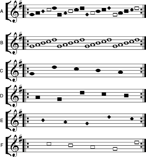

However, while this may work well for the performers, it is back-to-front for the audience. When an audience faces a stage to watch a live performance (see Figure 5.18), the instruments or singers producing the treble notes are on the left and the bass instruments or singers are on the right. This is the wrong way round in terms of the right-ear treble preference but the correct way round for observing the performers themselves. It is interesting to compare the normal concert hall layout as a listener with the experience of sitting in the audience area behind the orchestra, which is possible in halls such as the Royal Festival Hall in London. Unfortunately, this is not a test that can be carried out very satisfactorily, since it is not usually possible to sit far enough behind the players to gain as good an overall balance as can be obtained from the auditorium in front of the orchestra. It is, however, possible to experience this effect by turning round when listening to a good stereo recording over loudspeakers or by reversing the left and right channels.
5.5.4 Pitch Illusions
A pitch illusion, which has been compared with the continuous staircase pictures of M. C. Escher, has been demonstrated by Shepard (1964) and is often referred to as a “Shepard tone.” This illusion produces the sensation of an endless scale that ascends in semitone steps. After 12 semitone steps when the pitch has risen by one octave, the spectrum is identical to the starting spectrum, so the scale ascends but never climbs acoustically more than one octave. This stimulus is available on the CD recording of Houtsma et al. (1987) (and as tracks 68 and 69 on the accompanying CD). Figure 5.18 illustrates the spectral nature of the Shepard tone stimuli. Only the fundamental and harmonics that are multiple octaves above the fundamental are employed in the stimuli. The component frequencies of the Shepard tone can be represented as:
| f(Shepherd) = (2nf0) | (5.4) |
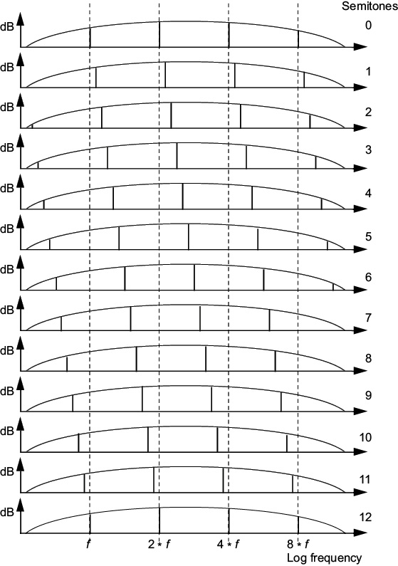

The amplitudes of the components are constrained within the curved envelope shown. Each time the tone moves up one semitone, the partials all move up by a twelfth of an octave, or one semitone. The upper harmonics become weaker and eventually disappear, and new lower harmonics appear and become stronger.
A musical example relating to the Shepard tone effect in which some pitch ambiguity is perceived by some listeners can be found in the pedal line starting at bar 31 of the Fantasia in G Minor (BWV 542) for organ by J. S. Bach (consider tracks 70–72 on the accompanying CD). These bars are reproduced in Figure 5.20 as an organ score in which the lower of the three staves is played on the pedals, while the upper two staves are played with the left and right hands.
The pedal line consists of a sequence of five descending scales with eight notes in each except the last. Each scale ends with an upward leap of a minor seventh, and the exact moment at which the upward leap occurs is often perceived with some ambiguity, even when listeners have the score in front of them. The strength of this effect depends on the particular stops used. This ambiguity is particularly common among listeners in the third bar of the extract, where the upward leap is often very strongly perceived as occurring one or even two notes later. This could be due to the entry of a new part in the left hand playing F3, which starts as the pedal part jumps up to written B♭3. (Reference to “written” B♭3 is made, since the 16′ rank provides the fundamental on the pedals, which sounds an octave lower than written pitch, as discussed in Section 5.4.)
The f0 components of these two notes, that is, F3 and B♭2, form the second and third harmonics of B♭1, which would have been the next sounding note of the pedal descending scale had it not jumped up an octave. At all the upward leaps in the descending pedal scales, the chord in the manual part changes from minor to major.
In bar 32, the left-hand change from E♭to E natural adds a member of the harmonic series (see Figure 3.3) of what would have been the next note (written C3) in the pedal scale had it not risen up the octave. E♭ is not a member of that harmonic series. The case is similar for the D♮ in the right hand in the third bar of the extract with the entry of the left-hand F3 and the left-hand C natural in the fourth bar. These entries of notes which are members of the harmonic series of what would have been the next note in the descending pedal scale had it not jumped up the octave serve to provide the perceived ambiguity in definition as to the exact instant at which the upward leap occurs.
The illusion produced by the combination of organ pipes to produce a sensation of pitch lower than any note actually sounding is also used in organ pedal resultant bass stops. These sound at 32′ (and very occasionally 64′), and their f0 values for bottom C are 16.25 Hz and 8.175 Hz, respectively. A resultant bass at 32′ pitch is formed by sounding together stops of 16′ and 102/3′, which form the second and third harmonics of the 32′ harmonic series (see Section 5.4). A 32′ stop perhaps labeled “acoustic bass” is a mutation stop of 102/3′, which when sounded with a 16′ rank produces a perceived pitch at 32′ (place theory of pitch perception from the second and third harmonics—see Chapter 3). A 64′ stop perhaps labeled “resultant bass” works similarly, sounding a 221/3′ rank with a 32′ rank.
The f0 value of the middle C of a 32′ stop (C2) is 65.4 Hz and thus its bottom note is two octaves below this (C0) with an f0 of (654/4) or 16.35 Hz. The f0 for the bottom note of a 64′ stop (C − 1) is 8.175 Hz, which is below the human hearing range but within the frequency range of difference frequencies that are perceived as beats (see Figure 2.6). Harmonics that are within the human hearing range will contribute to a perception of pitch at these f0 values, which are themselves below the frequency range of the hearing system. Organists will sometimes play fifths in the pedals to imitate this effect, particularly on the last note of a piece. However, the effect is not as satisfactory as that obtained with a properly voiced resultant bass stop, because the third harmonic (e.g., 102/3′) should be softer than the second harmonic (16′) for best effect.
Roederer (2008) describes an organ-based example to illustrate residue pitch, which constitutes a pitch illusion that is available as track 74 on the accompanying CD, while track 73 allows the chorale to be heard normally. The solo line of a chorale prelude—he suggests chorale number 40 from the Orgelbuchlein by J. S. Bach—is played using a number of mutation stops (see Section 5.5) if available (e.g., 8′, 4′, 22/3′, 2′, 13/5′, 11/3, 1) accompanied by 8′, 4′ in the left hand and 16′, 8′ in the pedal.
A musically trained audience should be asked to track the pitch of the melody and warned that timbre changes will occur. After playing a short snippet, play some more without the 8′, then without the 4′, then without the 2′, and finally without the 1′. What remains in the solo part is only mutation stops (i.e., those with a nonunison or nonoctave pitch relationship to the fundamental). Roederer suggests making
the audience aware of what was left in the upper voice and point out that the pitch of the written note was absent altogether (in any of its octaves)—they will find it hard to believe! A repetition of the experiment is likely to fail—because the audience will redirect their pitch processing strategies!
(Roederer, 2008, p. 154)
Experience shows that such an experiment relies on pitch context being established when using such stimuli, usually through the use of a known or continuing musical melody.
A musical illusion only works by virtue of establishing a strong expectation in the mind’s ear of the listener.
5.5.5 Assorted Auditory Illusions
In a similar vein to the Shepard tone pitch illusion described in Section 5.5.4, Risset (1986) introduced a rhythm-based phenomenon described as an eternal accelerando in which playing a rhythmic sequence is perceived as continually increasing in speed. Instead of using harmonics that are spaced in octaves as found in the Shepard tone (see Figure 5.19), a rhythmic sequence, along with copies of itself sped up to be in “tempo octaves” (twice as fast, four times as fast, eight times as fast, sixteen times as fast etc.) such that at the end of the sequence each has sped up by a factor of two (the tempo “octave”) so the sequence can be repeated. The amplitudes of the patterns at the low and high time extremes are gently faded such that the sequence toward the center of the set (the four-times-as-fast sequence in the example here) dominates what is perceived. If the sequences slow down rather than speed up, an eternal deccelerando can be produced. A practical implementation of the eternal accelerando is described by Stowell (2011), who provides audio examples (Risset, Rythm examples).
Beatboxing in which a single vocalist produces percussive sounds as well as vocal sounds, sometimes simultaneously, resulting in a sound in which the sung and percussive parts are heard as two separate lines, when in fact they are a single line interspersed with each other. We hear them as separate lines due to auditory streaming based on grouping by similarity (see Section 5.5.3). In addition, since a beatboxer can only produce a single line, the sung words are broken up by the percussive sounds. However, the sung lines are perceived as being continuous due to the fact that being masked by the percussive sounds, the perceptual system joins them up as if they were not broken up based on semantic context in terms of completing the phrases to make them meaningful. The percussive sounds produced by good well-established beatboxers can be extremely realistic; the key here is to ensure that the main acoustic cues for the percussion instruments are sufficiently clearly produced to work well in providing the main perceptual cues for the instruments themselves. Producing a convincing percussive sound is a nontrivial task, since it is being synthesized acoustically using the vocal tract, which itself is not a percussion instrument. On the other hand, the fact that the percussive sounds are emanating from the vocal tract means that the continuity illusion for the words works better than it would otherwise.
Throat singing, overtone singing or harmonic singing, as practiced by, for example, Mongolians, Tibetans, Inuits or Tuvans, is a form of auditory illusion in that it enables a tune to be vocalized while the main pitch of the note remains constant (or in some cases moves occasionally). The main pitch forms a drone in addition to the tune. The basic principle is that if individual harmonics are accentuated in amplitude sufficiently, that harmonic becomes a note in its own right; it “breaks away” from the holistic spectrum of its complex tone to be a sine wave that is heard as a second note. To achieve this, a very narrow band resonance is required from the vocal tract that can be moved in center frequency to be placed over a desired harmonic, in the same way that the formants modify the amplitudes of the harmonics of the vocal sound source in singing. A narrow-band spectrogram with a spectrum at the instant marked with the vertical line for a snippet of overtone singing is shown in Figure 4.38. The underlying drone note is F#2 with an f0 of 93 Hz. Since the underlying vowel is fixed, the overtones can be seen as any harmonics whose level (darkness of marking) varies, and in this case, it is approximately the twentieth to the twenty-fifth harmonics that are employed. The spectrum indicates how narrow the resonance is that enhances the overtone compared with the vowel formants at that instant.
References
ANSI, 1960. American Standard Acoustical Terminology. American National Standards Institute, New York.
Bregman, A. S., 1990. Auditory Scene Analysis. MIT Press, Cambridge.
Brookes, T., Tyrrell, A. M., and Howard, D. M., 2000. On the differences between conventional and auditory spectrograms of English consonants. Logoped. Phoniatr. Vocol. 25, 72–78.
Deutsch, D., 1974. An auditory illusion. Nature 251, 307–309.
Deutsch, D., 1975. Musical illusions. Sci. Am. 233, 92–104.
Deutsch, D., 1982. Grouping mechanisms in music. In: Deutsch, J. (ed.), The Psychology of Music. Academic Press, London, pp. 671–678.
Grey, J., 1977. Timbre discrimination in musical patterns. J. Acoust. Soc. Am. 64, 467–472.
Hall, D. E., 1991. Musical Acoustics: An Introduction, second edn. Wadsworth Publishing Company, Belmont.
Helmholtz, H.L.F. von, 1877. On the Sensations of Tone as a Physiological Basis for the Theory of Music, fourth edn. Dover, New York (1954 translation by A. J. Ellis).
Houtsma, A.J.M., Rossing, T. D., and Wagenaars, W. M., 1987. Auditory Demonstrations. Acoustical Society of America, New York (Philips compact disc No.1126–1061 and text).
Howard, D. M., 2005. Human hearing modeling real-time spectrography for visual feedback in singing training. Folia Phoniatr. Logo. 57 (5–6), 328–341.
Howard, D. M., Disley, A., and Hunt, A. D., 2007. Timbral adjectives for the control of a music synthesizer. In: Proceedings of the 19th International Congress on Acoustics, ICA-07, Paper MUS-07–004, 2–7 September, Madrid, Spain.
Howard, D. M., Hirson, A., Brookes, T., and Tyrrell, A. M., 1995. Spectrography of disputed speech samples by peripheral human hearing modeling. Forensic Linguist. 2 (1), 28–38.
Howard, D. M., and Tyrrell, A. M., 1997. Psychoacoustically informed spectrography and timbre. Organ. Sound 2 (2), 65–76.
Katz, R., 2007. Mastering Audio: The Art and the Science, second edn. Focal Press, Oxford.
Maes, J., 1996. The MiniDisk. Focal Press, Oxford.
Moore, B.C.J., 1996. Masking and the human auditory system. In: Gilchrist, N., and Grewin, C. (eds), Collected Papers on Digital Audio Bit-Rate Reduction. The Audio Engineering Society, New York, pp. 9–22.
Padgham, C. A., 1986. The Well-Tempered Organ. Positif Press, Oxford.
Pierce, J. R., 1992. The Science of Musical Sound (Scientific American Books), second edn. W. H. Freeman and Company, New York.
Pollard, H. F., and Jansson, E. V., 1982. A tristimulus method for the specification of musical timbre. Acustica 51, 162–171.
Rasch, R. A., and Plomp, R., 1982. The perception of musical tones. In: Deutsch, D. (ed.), The Psychology of Music. Academic Press, London, pp. 89–112.
Risset, J. C., 1986. Pitch and rhythm paradoxes: Comments on “Auditory paradox based on fractal waveform.” J. Acoust. Soc. Am. 80 (3), 961–962.
Risset, J. Rhythm examples. WWW-1: http://archive.org/details/risset1101
Roederer, J. G., 2008. Introduction to the Physics and Psychophysics of Music, 4th ed. Springer–Verlag, New York.Schoeder, M., 1986. Auditory paradox based on fractal waveform. J. Acoust. Soc. Am. 79, 186–189.
Scholes, P. A., 1970. The Oxford Companion to Music. Oxford University Press, London.
Shepard, R. N., 1964. Circularity in pitch judgement. J. Acoust. Soc. Am. 36, 2346–2353.
Stowell, D., 2011. Scheduling and composing with Risset eternal accelerando rhythms. In: Proceedings of the International Computer Music Conference 2011, University of Huddersfield, UK, 31 July–5 August 2011, pp. 474–477.
Sumner, W. L., 1975. The Organ. MacDonald and Company, London.
Sundberg, J., 1991. The Science of Musical Sounds. Academic Press, San Diego.