2

Creating the Past, Present, and Future with Random Walks

John Manslow

2.1  Introduction

Randomness plays an important role in many games by adding replay value and forcing the player to adapt to unpredictable events. It often takes the form of variables with values that change gradually but randomly with time and hence perform what are technically known as random walks. Such variables might affect visibility or cloud cover in a weather simulation, the mood of an NPC, the loyalty of a political faction, or the price of a commodity. This chapter will describe the statistical properties of normally distributed random walks and will show how they can be shaped and manipulated so that they remain unpredictable while also being subject to scripted constraints and responsive to player interaction.

We begin by describing how to generate a simple random walk and discuss some of its limitations. We then show how to overcome those limitations using the walk’s statistical properties to efficiently sample from it at arbitrary points in its past and future. Next, we discuss how to fix the values of the walk at specific points in time, how to control the general shape of the movement of the walk between them, and how to limit the walk to a specific range of values. Finally, we describe how to generate random walks with arbitrary probability distributions and to allow for player interaction. The book’s web site contains spreadsheets and C++ source code for all the techniques that are described in this chapter.

2.2  Problems with a Basic Random Walk

One simple way to generate a random walk is to initialize a variable, say x, to some desired starting value x₀, and then, on each step of the simulation of the game world, add a sample from a normal distribution (a bell curve). This process is fast and efficient and produces values of x that start at x₀ and then randomly wander around, perhaps ending up a long way from the starting point or perhaps returning to a point close to it.

This approach is not without its problems, however. For example, how can we work out what the value of x will be two days from now? Equivalently, what value should x be at right now, given that the player last observed it having a particular value two days ago? Perhaps we are simulating the prices of commodities in a large procedurally generated universe, and the player has just returned to a planet that they last visited two days ago. This is the problem of extrapolating a random walk.

2.3  Solving the Extrapolation Problem Using Statistical Methods

One way to solve the extrapolation problem is to quickly simulate the missing part of the random walk. However, this might be computationally infeasible or undesirable, particularly if we are modeling a large number of random walks simultaneously, as might be the case if they represent prices in a virtual economy. Fortunately, we can use statistical methods to work out exactly how x will be distributed two days after it was last observed based only on the last observed value. Specifically, the central limit theorem tells us that if x had the value x₀ at time t₀, then at time t, x will be distributed as

$p\left(x\right)\sim N\left(x_0,\left(t-t_0\right){\text{σ}}_{xx}^2\right)$

(2.1)

This is a normal distribution with the following two characteristics: it has mean x₀, which is the last observed value; and variance (t − t₀)σ²_xx, where t − t₀ is the time since the last observation; and σ²_xx is a parameter that controls how quickly the walk can wander away from the starting point. In fact, since the distribution is normal, we know that x will lie in a range of approximately $x_0\pm 1.96\sqrt{(t-t_0){\text{σ}}_{xx}^2}$ about 95% of the time. Figure 2.1a shows a random walk generated using Equation 2.1 with x₀ equal to 90 and σ²_xx equal to one. Figure 2.1b shows how increasing the value of σ²_xx to five makes the walk wander about much more rapidly.

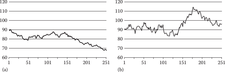
Figure 2.1
(a) shows 250 steps of a random walk generated using the extrapolation equation and (b) shows the effect of increasing σ²_xx.

Of course, we need to select a specific value for x, and that can be done by sampling from p(x). Although this produces a value of x that is technically not the same as the one that would have been produced by simulating two days’ worth of random walk, it is impossible for the player to tell the difference because the true value and the sampled value have identical statistical properties given the player’s limited state of knowledge about how the numbers are generated.

Equation 2.1 actually provides us with a much better way of generating random walks than the naive approach that was mentioned earlier. In particular, because t − t₀ represents the time between successive samples, it allows us to update the random walk in a way that is invariant to changes in the real times of steps in the simulation of the game world; the statistical properties of the walk will remain the same even if the times between updates are irregular or different on different platforms.

To generate a random walk using Equation 2.1, first pick an initial value for x₀ for use in p(x), and then sample from p(x) to get the next value, x₁. The value x₁ can then be used in place of x₀ in p(x), and x₂ can be sampled from p(x). Next, use x₂ in place of x₁ in p(x) and sample x₃, and so on. In each case, the time interval should be the time between the observations of the random walk and hence might be the times between updates to the game world but might also be arbitrary and irregular intervals if the player does not observe the value of the walk on every tick of the game engine.

An interesting feature of Equation 2.1 is that it is time reversible and hence can be used to generate values of x in the past just as easily as ones in the future. Consider if a player visits a planet for the first time and needs to see a history of the price of a commodity. Equation 2.1 can be used to generate a sequence of samples that represent the price history. This is done in exactly the same way as when samples are generated forward in time except that x₁ would be interpreted as preceding x₀, x₂ would be interpreted as preceding x₁, and so on.

Although having the ability to extrapolate random walks forward and backward in time is extremely useful, we often need to do more. What happens, for example, if the player has observed the value of a variable but we need to make sure that it has some other specific value in one hour from now? This situation might arise if a prescripted event is due to occur—perhaps a war will affect commodity prices, or there will be a thunderstorm for which we need thick cloud cover. Since we now have two fixed points on the walk—the most recently observed value and a specified future value—it is no longer good enough to be able to extrapolate—we must interpolate.

2.4  Using Interpolation to Walk toward a Fixed Point

Now that we can generate samples from a random walk that are consistent with a single fixed value, we have everything we need to interpolate between two fixed values—we just need to generate samples that are consistent with both. We do this by calculating the probability distributions for x with respect to each of the fixed values and then multiply them together. As Equation 2.1 represents a normal distribution, we can write down the probability distribution for interpolated points quite easily:

$$\begin{gathered} p\left(x\right)~N(\left(\frac{x_0}{\left(t-t_0\right){\text{σ}}_{xx}^2}+\frac{x_n}{\left(t_n-t\right){\text{σ}}_{xx}^2}\right)/\left(\frac{1}{\left(t-t_0\right){\text{σ}}_{xx}^2}+\frac{1}{\left(t_n-t\right){\text{σ}}_{xx}^2}\right), \\ 1/\left(\frac{1}{\left(t-t_0\right){\text{σ}}_{xx}^2}+\frac{1}{\left(t_n-t\right){\text{σ}}_{xx}^2}\right)) \end{gathered}$$

(2.2)

Here x₀ is the first specified value, which occurs at time t₀; x_n is the second, which occurs at t_n; and x is the interpolated value of the walk at any time t. As before, in order to obtain a specific value for x, we need to sample from this distribution. Interpolated values of x are guaranteed to start at x₀ at time t₀, to randomly wander around between t₀ and t_n, and to converge to x_n at time t_n. Interpolation therefore makes it possible to precisely determine the value of the walk at specific points in time while leaving it free to wander about in between.

To generate a walk using Equation 2.2, use x₀ and x_n to sample from p(x) to generate the next value of x and x₁. Next, use x₁ in place of x₀ and sample again from p(x) to generate x₂, and so on—this can be done either forward or backward in time. The interpolation equation has fractal properties and will always reveal more detail no matter how small the interpolated interval. This means that it can be applied recursively to solve problems like allowing the player to see a 25-year history of the price of a particular commodity while also allowing him to zoom in on any part of the history to reveal submillisecond price movements.

2.5  Restricting the Walk to a Fixed Range of Values

One potentially undesirable feature of the random walk that has been described so far is that, given enough time, it might wander arbitrarily far from its starting point. In practice, however, we usually want it to take on some range of reasonable values, and this can easily be done by adding a statistical constraint that specifies that the values of x must, over an infinite amount of time, follow a particular probability distribution. If we choose a normal distribution with mean x* and variance σ^*2 to keep the math simple, the equation for extrapolating becomes

$p\left(x\right)\sim N\left(\left(\frac{x_0}{\left(t-t_0\right){\text{σ}}_{xx}^2}+\frac{x^{\ast }}{{\text{σ}}^{\ast 2}}\right)/\left(\frac{1}{\left(t-t_0\right){\text{σ}}_{xx}^2}+\frac{1}{{\text{σ}}^{\ast 2}}\right),1/\left(\frac{1}{\left(t-t_0\right){\text{σ}}_{xx}^2}+\frac{1}{{\text{σ}}^{\ast 2}}\right)\right)$

(2.3)

and the equation for interpolating becomes

$p\left(x\right)~N\left(\frac{\left(\frac{x_0}{\left(t-t_0\right){\text{σ}}_{xx}^2}+\frac{x^{\ast }}{{\text{σ}}^{\ast 2}}+\frac{x_n}{\left(t_n-t\right){\text{σ}}_{xx}^2}\right)}{\left(\frac{1}{\left(t-t_0\right){\text{σ}}_{xx}^2}+\frac{1}{{\text{σ}}^{\ast 2}}+\frac{1}{\left(t_n-t\right){\text{σ}}_{xx}^2}\right)},1/\left(\frac{1}{\left(t-t_0\right){\text{σ}}_{xx}^2}+\frac{1}{{\text{σ}}^{\ast 2}}+\frac{1}{\left(t_n-t\right){\text{σ}}_{xx}^2}\right)\right)\text{}$

(2.4)

A walk generated according to these equations is subject to a soft bound in the sense that it will lie in the range $x^{\ast }\pm 1.96\sqrt{{\text{σ}}^{\ast 2}}$ about 95% of the time but will occasionally wander a little further, exceeding $x^{\ast }\pm 6.11\sqrt{{\text{σ}}^{\ast 2}}$ with a probability of less than one in a billion. Figure 2.2a shows a random walk generated according to Equation 2.3 with x* equal to 90 and σ^*2 equal to 100.

If it is necessary to be absolutely certain that the walk will stay between fixed bounds, then it is better to use the unconstrained extrapolation and interpolation equations and postprocess the values they generate. If this is done by reflecting the walk off the bounds whenever it encounters them, the walk will retain the important statistical property that its behavior is invariant to the time steps that are used to generate it. To see how this works in practice, consider generating a random walk that must be constrained to lie between zero and one.

This can be done by generating a dummy variable x* using the unconstrained extrapolation and interpolation equations but presenting a value x to the player that is derived according to the following rules:

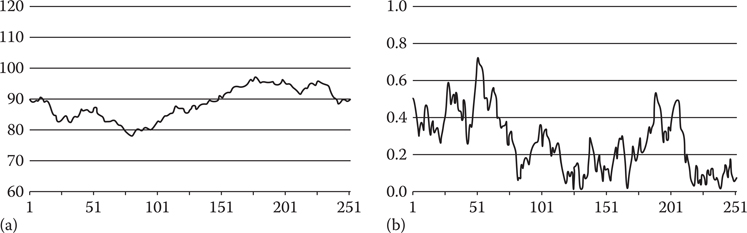
Figure 2.2
(a) shows a random walk that is soft bounded to have a normal distribution with x* = 90 and σ^*2 = 100 and (b) shows a random walk that is hard bounded to lie between zero and one.

x will perform the required random walk between the bounds zero and one, and in the long term will tend toward a uniform distribution. Figure 2.2b shows a random walk between the bounds zero and one that was generated using this technique. If we simply require x to be nonnegative, it is sufficient to take the absolute value of x*; doing so will produce a random walk that is always nonnegative that will also, in the long term, tend toward a uniform distribution.

2.6  Manipulating and Shaping the Walk with Additive Functions

We have so far described how a random walk can be manipulated by using the interpolation equation with one or more fixed points. Interpolation guarantees that the walk will pass through the required points but it gives us no control over what it does in between—whether it follows roughly a straight line, roughly a curve, or makes multiple sudden jumps. Sometimes we want exactly that kind of control, and one way to achieve it is simply to add the random walk to another function that provides the basic form of the walk that we want. In this way, the random walk is just adding random variability to disguise the simple underlying form.

Consider a game where we have a commodity with a price of 90 credits that must rise to 110 credits in one hour from now. We could simply do this by using the interpolation equation and letting the walk find its own way between the two fixed price points, as shown in Figure 2.3a. Alternatively, we could choose a function that starts at 90 credits and rises to 110 credits and provides us with the basic shape of the movement we want and add to it a random walk that is bounded by the interpolation equation to start and end at zero.

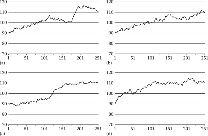
Figure 2.3
(a) shows the result of using the basic interpolation equation to generate a random walk from 90 to 110 in 250 steps, (b) shows the result of using a linear function to shape the walk, (c) shows the result of using the smoothstep function, and (d) shows the result of using the quarter circle function.

For example, we might want the price to move roughly linearly between the fixed points so we would use the linear function

$x=90\left(1-t\right)+110t$

(2.5)

to provide the basic shape. Here, for convenience, t has been scaled so that it has the value zero at the start of the hour and one at the end. By adding the random walk to values of x generated by this formula and using the interpolation formula to generate the random walk in such a way that it starts and ends at zero, the sum of x and the random walk will be 90 at the start of the hour, 110 at the end, and move roughly linearly in between but with some random variation, as shown in Figure 2.3b.

Of course, we do not always have to use a linear function to provide the basic form. Other useful functions are the step function, which produces a sudden jump, the smoothstep function

$x=90+20\left(3t^2-2t^3\right)$

(2.6)

which provides a smoothly curving transition, and the quarter circle function

$x=90+20\sqrt{1-{\left(1-t\right)}^2}$

(2.7)

which rises rapidly at first and then levels out. Random walks based on the smoothstep and quarter circle functions are shown in Figure 2.3c and d respectively.

2.7  Using Additive Functions to Allow for Player Interaction

We now know how to extrapolate and interpolate random walks and bend and manipulate them in interesting ways, but how can we make them interactive so that the player can influence where they go? Fortunately, player interaction is just another way in which random walks are manipulated and hence all of the techniques that have already been described can be used to produce player interaction.

For example, the player might start a research program that produces a 25% reduction in the basic cost of a particular weapon class over the course of 15 minutes. This effect could be produced by simulating the price using a random walk with zero mean added to a function that represents the average price, which declines by 25% during the course of the research program. This will produce a price that randomly wanders around but is typically 25% lower once the research program has completed than it was before it was started.

Similarly, a player might sell a large quantity of a particular commodity, and we might want to simulate the effect of a temporary excess of supply over demand by showing a temporary reduction in its price. This could be done either by recording an observation of an artificially reduced price immediately after the sale and generating future prices by extrapolation or by subtracting an exponentially decaying function from the commodity’s price and allowing the randomness of the walk to hide the function’s simple form.

In the case of the research program, we must permanently record the action of the player, and its effect on price because the effect was permanent. In the case of the excess of supply over demand, the effect is essentially temporary because the exponential decay will ensure that it will eventually become so small that it can be ignored, at which point the game can forget about it unless it might need to create a price history at some point in the future.

2.8  Combining Walks to Simulate Dependent Variables

We have so far discussed how to generate independent random walks and provided a simple set of tools for controlling and manipulating them. In practice, we might need to generate random walks that are in some way related: perhaps we need two random walks that tend to go up and down at the same time, or one that tends to go up when another goes down or vice versa. These effects can easily be achieved by adding and multiplying random walks together and through the use of dummy variables.

Imagine that we need to simulate the prices of electronics and robotics products. Since electronics products are a core component of robotics products, we would expect the price of robotics products to increase if the price of electronics products increased—but not for either price to track the other exactly. This effect can be achieved by modeling the price of electronics products using a random walk and then using another random walk to model a dummy variable that represents either the difference in the prices of electronics and robotics products or their ratio.

If we decide to use a dummy variable to represent the difference between the prices, we could use a random walk with an x* of 100 and σ^*2 of 100 to model the price of electronics products and a walk with x* of 25 and σ^*2 of 100 to model the difference in the price of electronics products and robotics products. Since the price of robotics products would be the sum of the values of these two random walks, it would itself be a random walk, and it would have an x* of 125 and an σ^*2 of 200 and would tend to increase and decrease with the prices of electronics products, as shown in Figure 2.4.

Combinations of random walks can be made arbitrarily complex. The price of a spacecraft, for example, could be a weighted sum of the prices of its various components plus the value of a dummy variable that represents the deviation of the actual sale price from the total cost of its components. In general, if a random walk is formed by a sum of N component random walks x₁…x_N with means x*₁…x*_N and variances σ^*₁²…σ^*_N², which have weights w₁…w_N in the sum, it will have mean

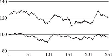
Figure 2.4
The lower random walk has x* = 100 and σ^*2 = 100 and represents the price of electronics products. The upper random walk is the sum of the lower random walk and another with x* = 25 and σ^*2 = 100 and represents the price of robotics products.

$x^{\ast }=\sum _{n=1}^N{w}_n{x}_n^{\ast }$

(2.8)

and variance

${\text{σ}}^{\ast 2}=\sum _{n=1}^N{w}_n^2{\text{σ}}_n^{\ast 2}$

(2.9)

It could be the case that the player can observe the values of all, some, or none of the components in the sum. We might, for example, want to make the prices of a commodity in a space simulation more similar in star systems that are closer together, and one way to do that is to use a dummy variable in each system to represent a dummy price that the player cannot observe. The price that the player would see in any particular system would then be the weighted sum of the dummy prices of neighboring systems with larger weights being assigned to closer systems. It is interesting to note that if one of the components in Equation 2.8 has a negative weight, then it produces a negative correlation; that is, when its value increases, it will tend to reduce the value of the sum. This can be useful when walks represent mutually competing interests such as the strengths of warring empires.

2.9  Generating Walks with Different Probability Distributions

If a random walk is generated according to the soft-bounded extrapolation equation, the values it takes will, over a long period of time, have a normal distribution with mean x* and variance σ^*2. This is perfect for most applications, but we will occasionally want to generate a walk with a different distribution. For example, share prices have been modeled using log-normal distributions, and we can easily generate a log-normally distributed random walk by interpreting the extrapolation equation as modeling the natural logarithm of the share price and producing the actual price by applying the exponential function.

More generally, the inverse transformation method is often used to convert a random variable that is uniformly distributed between zero and one to another random variable with a particular target distribution by applying a nonlinear transformation. For example, taking the natural logarithm of a random variable that is uniformly distributed between zero and one produces a random variable that has an exponential distribution that can be used to realistically model the times between random events.

Although the random walks that have been described in this chapter have normal distributions, they can be made uniformly distributed by hard bounding them to a fixed interval, as was described earlier, or by transforming them using the cumulative normal distribution function. Specifically, if a sample x from a random walk has mean x* and variance σ^*2, we can compute the variable

$y=F\left(x,x^{\ast },{\text{σ}}^{\ast 2}\right)$

(2.10)

where F is the cumulative normal distribution function. The variable y will be uniformly distributed between zero and one and hence can be used with the inverse transformation method to generate random walks with a wide range of distributions. For example, a linear transformation of y can be used to produce a random walk that is uniformly distributed over an arbitrary range of values, while taking the natural logarithm produces a walk with an exponential distribution. It should be noted that, when the inverse transformation method is used to change a random walk’s distribution, the sizes of the steps taken by the walk will not be independent of its value. A walk that is bounded by the inverse transformation method to lie in the range zero to one, for example, will take smaller steps when its value is close to its bounds than when it is far from them.

2.10  Solving the Persistence Problem with Procedural Generation

At the heart of a computer-generated random walk lies a random number generator that can be made to produce and reproduce a specific sequence of numbers by applying a seed. By recording the seed values that were used in constructing parts of a random walk, those parts can be exactly reconstructed if and when required. For example, if a player visited a planet for the first time and looked at the history of the price of a commodity over the last year, that history could be created by seeding the random number generator with the time of the player’s visit and then applying the extrapolation equation backward in time. If the player returned to the planet a couple of months later and looked at the same history, it could easily be reconstructed based only on the original seed, and hence the history itself would not need to be stored. This is a major benefit, particularly in large open world games that contain many random walks with detailed and observable histories.

2.11  Conclusion

This chapter has provided a selection of simple but powerful techniques for generating and manipulating random walks. The techniques make it possible to exploit the unpredictability and replay value that randomness adds while also providing the control that is necessary to allow it to be both scripted and interactive when necessary. Spreadsheets and C++ classes that demonstrate the key concepts that are described in this chapter have been provided to make it as easy as possible to apply them in practice.