15

Steering against Complex Vehicles in Assassin’s Creed Syndicate

Eric Martel

15.1  Introduction

The different worlds in which videogames exist are becoming more and more complex with each passing day. One of the principal reasons NPCs appear intelligent is their ability to properly understand their environments and adjust their behaviors accordingly. On Assassin’s Creed Syndicate, part of the mandate for the AI team was to support horse-drawn carriages at every level for the NPCs. For this reason, we adapted the NPCs’ steering behaviors to navigate around a convex hull representing the vehicles instead of using a traditional radius-based avoidance. We succeeded in building general-purpose object avoidance behavior for virtually any obstacle shape.

A real-time JavaScript implementation of this material is available at http://steering.ericmartel.com should you wish to experiment with the solution as you progress throughout the article.

15.2  Challenges and Initial Approaches

Most object avoidance steering behaviors are implemented by avoiding circles or ellipses (Reynolds 1999, Buckland 2005). In our case, the vehicles were elongated to such an extent that even by building the tightest possible ellipse encompassing the entire bounding box of the vehicle, we ended up with unrealistic paths from our NPC agents. They would venture far away from the sides of the vehicle despite having a straight clear path to their destination. We wanted NPCs to be able to walk right next to a vehicle like a person in real life would. Note that the solution provided here was only for the navigation of humanoids. Steering behaviors for the vehicles themselves are handled differently and will not be described here.

15.2.1  Navigation Mesh Patching

From the very beginning, we decided that the NPCs should reject a path request if it is physically impossible for them to pass when a vehicle is blocking their way. This implies that, in these situations, changes needed to be made to the navigation mesh. Considering that many vehicles can stop at the same time, each forcing the navigation mesh to be recomputed, we decided to time slice the process. In other words, several frames might be required before the pathfinder properly handles all the stopping vehicles. To avoid having NPCs run against them, a signal system is used to turn on the vehicle in the obstacle avoidance system as soon as it moves and then turn it off as soon as the navigation mesh underneath it is updated. Unfortunately, the steering technique described here will not identify situations where vehicles will completely block a path. The algorithms could be adapted, if required, to test the intersection with the navigation mesh outside edges.

15.2.2  Obstacle Avoidance

Classical obstacle avoidance provides an agent with a lateral pushing force and a braking force, allowing the agent to reorient itself and clear obstacles without bumping into them, as shown in Figure 15.1. Given circular or even spherical obstacles, this is pretty straightforward.

15.2.3  Representation Comparison

Starting off with our existing technology, we experimented with various representations. The first implementation used a circle-based avoidance, increasing the diameter of the circle to encompass the entire vehicle. Although this worked, it did not look realistic enough; agents would walk far away from the sides of a vehicle to avoid it, as is shown in Figure 15.2.

To mitigate the wide avoidance paths, we considered modifying the circular obstacles into ellipses. Ellipses are slightly more complicated to use for obstacle avoidance, as their orientation needs to be taken into account when calculating the lateral push and the breaking factor. Unfortunately, as seen in Figure 15.3, even without implementing them, we knew we would not get the kind of results needed, as the sides were still too wide. Another solution had to be created.

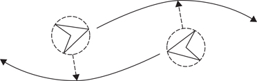
Figure 15.1
Circle-based obstacle avoidance between two agents.

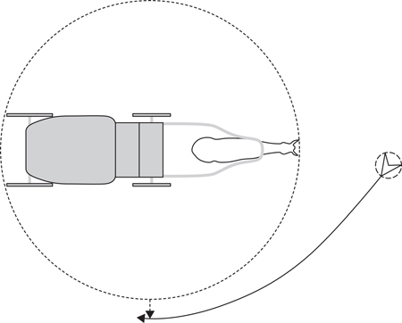
Figure 15.2
Circle-based representation of an elongated obstacle.

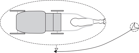
Figure 15.3
Ellipse-based representation of an elongated obstacle.

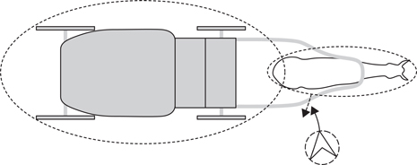
Figure 15.4
Multiple ellipses representing an elongated obstacle.

We considered representing each portion of the vehicle as an ellipse, as it would allow us to represent our collision volumes more accurately. The problem with this representation, as depicted in Figure 15.4, is that by using multiple ellipses, a nook is created between the horse and the carriage. Without handling multiple obstacles at the same time, one risks having the agent oscillate between both parts and then get stuck in the middle.

15.3  Convex Hull Generation

The best representation of the vehicle we could conceive was a convex hull, as it could wrap around all of the subparts of the vehicle without creating any concave sections. This would allow the NPC to steer against the horse-drawn carriage as if it were a single uniform obstacle.

Our obstacles are made out of multiple rigid bodies, each representing a subpart of the vehicle. Some carriages have two horses, others a single one, and after firefights or accidents, a carriage can be left with no horse at all.

15.3.1  Rigid Body Simplification

In order to reduce the number of elements in our data structures, we simplified the representation of our rigid bodies to 2D object-oriented bounding boxes (OOBB). Since our NPCs are not able to fly, we could forgo the complexity of 3D avoidance. By flattening down the 3D OOBB encompassing the rigid bodies provided by our physics engine, we managed to have an accurate representation of our vehicle from top view. In the following examples, we have omitted adding yaw or roll to the subparts (Figure 15.5).

When computing circle-based avoidance, it is easy to simply add the radius of the agent to the repulsion vector, thus making sure it clears the obstacle completely. In our case, we simply grew the shapes of our OOBB of half the width of the characters, making sure that any position outside that shape could accommodate an NPC without resulting in a collision. From that point on, NPCs are navigating as a single point against the expanded geometry of the vehicles.

15.3.2  Cases to Solve

We identified three main situations that need to be handled, pictured in Figure 15.6, ordered from most to least frequent. The most interesting case is the one where shapes are partially overlapping (Figure 15.6a). The algorithm to solve this case is provided in Section 15.3.4.

Two shapes are disconnected when all of the vertices of the first shape are explored finding that none of its edge segments intersect with the second shape, and that none of the vertices of either shape lie inside the other. When shapes are disconnected, we decided to simply merge the two closest edges. In our example from Figure 15.6b, the edges “AD” and “BC” would be removed. Starting from the first vertex of the bottom shape, we iterate on the shape until we reach vertex “A,” then switch shape from vertex “B.” The process continues until we reach vertex “C” at which point we go back to the initial shape from “D.” The operation is complete once we loop back to the first vertex. As long as our vertices are kept in clockwise order, performing this operation remains trivial.

A case that we did not tackle in our implementation is demonstrated in Figure 15.7, where the shapes loop, creating two contours. Given the shape of our entities, this is simply not required. It would be easy to adapt the algorithm to support multiple contours with a single convex hull built around the outer contour.

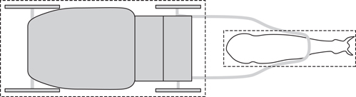
Figure 15.5
Object-oriented bounding boxes representing the obstacle subparts.

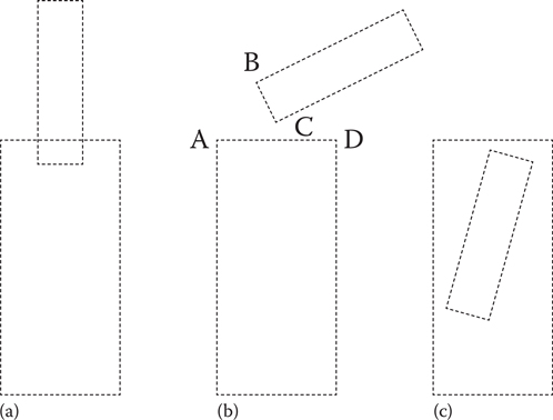
Figure 15.6
The various cases that need to be supported when joining shapes, from left to right: (a) partial overlap, (b) disconnection, and (c) complete overlap.

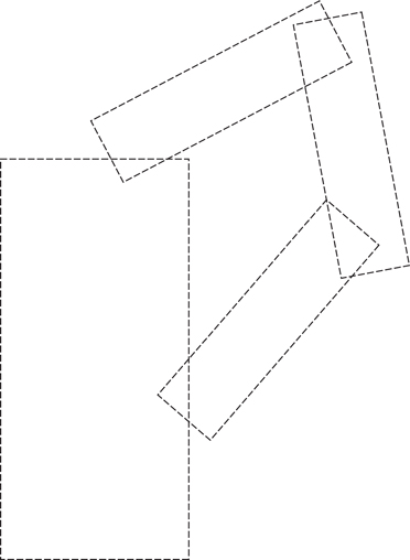
Figure 15.7
Additional case. When enough subparts are present or when the subparts themselves are concave polygons, multiple contours have to be handled.

15.3.3  Building the Contour

Before diving into the construction of the contour, the following algorithms were chosen in order to keep things simple, understandable, and to make most of the intermediate data Vuseful. There might be specialized algorithms that are more efficient in your case, feel free to replace them.

First, let us take a look at a useful function, as shown in Listing 15.1, that will be used on multiple occasions in the code. This method simply moves an index left or right of a current value, while wrapping around when either ends of the list are reached. This will allow us to avoid having to include modulo operations everywhere in the code. Although adding listSize to currentValue might look atypical at first, it allows us to handle negative increment values which in turn make it possible to iterate left and right in the list.

What follows next is an example of how the algorithm merges and constructs intersecting shapes. As pictured in Figure 15.8, we start from a vertex outside of the second shape, and we iterate in a clockwise fashion as long as we are not intersecting with any edge of the second shape. When finding an intersection, we simply insert the intersection point and swap both shapes as we are now exploring the second shape looking for intersections until we loop around.

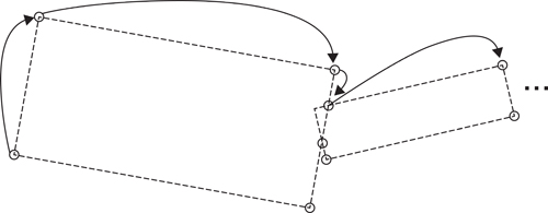
Figure 15.8
Algorithm for intersecting shapes. Merging the shapes by iterating over them, creating ­vertices on intersections.

The code in Listing 15.2 merges shapes one at a time. Instead of handling the complexity of merging n shapes at the same time, shapes are added to a contour that grows with every subpart added.

For the full source code, please visit the article’s website listed in Section 15.1. Consider that firstOutsideVtx could fail if all the vertices of currVtx are inside altVtx as seen in Figure 15.6c. If the while loop completes and mergedContour is the same size as currVtx, either no intersections happened or all the vertices of currVtx are inside altVtx, which is easy to test.

15.3.4  Expanding the Convex Hull

At this point, we now have a list of vertices ordered clockwise that might, or might not, represent the convex hull. For the polygon to represent a convex hull, all of its interior angles need to be lower or equal to 180°. If an angle is greater than 180, it is easily solved by removing the vertex and letting its two neighbors connect to one another. Removing it from the array corrects this because of the use of ordered list of vertices. Listing 15.3 describes how this can be accomplished with a few lines of code by using the Z value of the cross product to determine on which side the angle is heading. It is important to always step back one vertex after the removal operation, as there is no guarantee that the newly created angle is not greater than 180° as well.

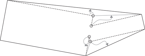
Figure 15.9
Removing vertices that make the polygon concave.

As can be seen in Figure 15.9, it is as if we are folding out the pointy ends of the polygon until we end up with a convex hull.

15.4  Obstacle Avoidance

Now that the geometry is constructed, we can go about shaping the NPCs’ behavior around it. This implies that we must first find out if our current position or our destination is inside the convex hull. Any position between the vehicle’s OOBB and the convex hull is actually a walkable area. If neither position is located inside the convex hull, we must then check if there is a potential collision between the NPC and the obstacle.

15.4.1  Obstacle Detection

Most steering behavior systems use a feeler system to detect potential incoming obstacles. In our case, to accelerate and parallelize the system, we utilize axis-aligned bounding boxes that are sent to the physics system. The physics system then matches pairs that are intersecting and allows us to easily know, from the gameplay code, which other entities to test for avoidance.

Once we know we have a potential collision, we can determine if either the start or end positions are inside the convex hull. Using a method similar to Listing 15.4, that is by counting the number of intersections between a segment starting at the tested position and ending at an arbitrary position outside of the polygon and with the polygon itself, we can determine whether or not we are located outside of the shape. An odd number of intersections signals that the position is inside. Otherwise it is outside, as our segment went in and out of the shape an even number of times.

For an example of collectIntersections or how to check for intersections between segments, feel free to refer to the website listed in the introduction.

15.4.2  Movement around the Convex Hull

When we know that both our current position and destination are outside of the convex hull, a simple intersection check using a segment between both of these positions and the convex hull can confirm whether or not the NPCs are clearing the shape. Having expanded the shape by the radius of the agent guarantees us that if there is no intersection; the NPC is free to go in straight line and will not collide with the obstacle. If the agents have different radii, it is also possible to simply offset the intersection check by the radius of the agent, either on its right or left vector, depending on the relative side of the obstacle.

If an intersection is detected, the NPC must avoid the obstacle. Depending on the relative velocities, you might want to control on which side the avoidance occurs. For the purpose of demonstration, we define that our objective is to minimize the angle between our avoidance vector and our current intended heading.

From the intersection detection, we can extract the vertex information from both ends of the segment with which we intersect. As the vertices are in clockwise order, we know that we can explore their neighbors by decreasing the index of the start vertex to go on the right, and increase the index of the end vertex to go on the left. We are looking for the furthest vertex to which we can draw a straight line without intersecting with the other segments of the convex hull, which also minimizes the angle difference with the intended direction. In Figure 15.10, the end vertex of the intersected segment happened to be the best vertex matching this criterion, as its next neighbor would cause an intersection with the convex hull, and the exploration on the right leads to a greater angle difference.

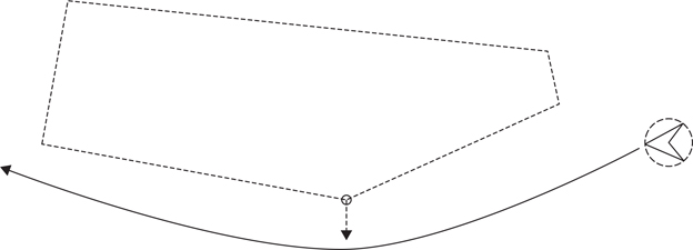
Figure 15.10
Obstacle avoidance when both the start and end points are outside of the obstacle.

15.4.3  Movement into the Convex Hull

In the game, NPCs are able to interact with vehicles even while in movement. For this reason, it can happen that their interaction point lies inside the convex hull. In this case, two situations can occur: either the segment between the character and its destination intersects with the contour, or it does not. The convex hull being only a virtual shell around the vehicle does not prevent the agent from going through it, so if no intersection is found with the contour, the NPC can simply walk in straight line to its destination, as shown in Figure 15.11.

The real challenge when an intersection is detected is to find the right direction to send the NPC, since if it walks around the obstacle, it will eventually clear the contour and enter the convex hull. A solution for this problem is to find the edge of the convex hull that is closest to the destination. Doing this, we have two vertices that represent an entry point to the convex hull. By reusing part of the solution in Section 15.4.2, we iterate over the convex hull from our initial intersection toward the two vertices we found earlier. We are trying to find the closest vertex to us that minimizes the distance between it and one of the two vertices without intersecting with the contour. This distance can be calculated by summing the length of the edges of the convex hull as we are moving in either direction. As we progress, the edge of the convex hull that connects with space where the destination lies will be reached.

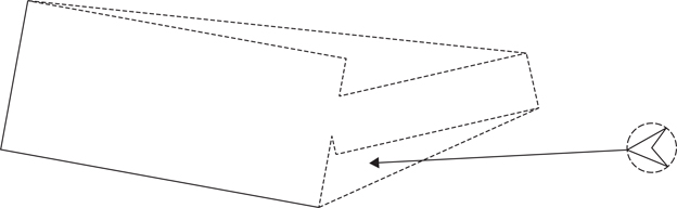
Figure 15.11
Obstacle avoidance when the destination is inside the convex hull.

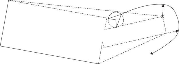
Figure 15.12
Obstacle avoidance when the agent is inside the convex hull.

At this point, we know the destination is in a polygon, and we are about to enter it. Unfortunately, it is possible that the shape between the contour and the convex hull is a concave polygon. No trivial solution is available, but two well-known options are available to you. Either the NPC “hugs the walls” of the contour by following its neighbor edge until it gets a straight line between itself and the destination or the space is triangulated allowing the algorithm to perform a local path planning request, which will be described in Section 15.5.1.

15.4.4  Movement Out of the Convex Hull

When the agent lies inside the hull, we can deduce the way to exit the shape by reversing the operations of those proposed in Section 15.4.3. We first make the NPC navigate out of the polygon representing the difference between the contour and the convex hull. Once outside, the methods described in Sections 15.4.2 and 15.4.3 should be applied, as the destination will either be inside or outside of the convex hull (Figure 15.12).

15.5  Pushing It Further

The following suggestions are not required to make steering against arbitrary shapes work, but it could improve the quality of your results.

15.5.1  Triangulation from Convex Hull Data

When taking a closer look at Figure 15.9, one might notice that as we removed the vertices, we were actually adding triangles to the contour to push it outward and create the convex hull. As pictured in Figure 15.13, a simple adjustment to the algorithm can push the triangle data as the vertices are popped in order to create a simple local navigation mesh. Local path planning can be used to guide the obstacle avoidance going in and out, generate optimal paths, and simplify the logic required when positions are inside the convex hull.

15.5.2  Velocity Prediction

Given that the state of these obstacles are volatile, we did not spend the time to model the velocity of the subparts of the vehicle but only the obstacle’s velocity. If you were to model a giant robotic space snake, then allowing NPCs to predict where the tail will be ahead of time may be required, but it comes at the expense of computing the position of the subparts in advance.

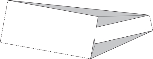
Figure 15.13
Adapting the convex hull generation algorithm to produce a navigation mesh inside the convex hull.

In most cases, mimicking what humans would do gives the best results. In the case of our game, an agent crossing a moving vehicle will often try to go behind it. Modeling whether the agent is going roughly in the same direction, in opposite direction, or in a perpendicular direction will allow you to give more diversity in which vertex from the convex hull you want to target and how much you want to modulate the braking factor.

15.6  Conclusion

Converting obstacles’ shapes to a convex hull really improved the quality of the navigation of our NPCs around them. This solution is also generic enough to be applied to any rigid body, from vehicles to destructible environments. Performance wise, by lazily evaluating the shape of the rigid body and caching the results for all surrounding characters, we managed to get the best of both worlds.

References

Buckland, M. 2005. Programming Game AI by Example. Plano, TX: Wordware Publishing.

Reynolds, C. W. 1999. Steering behaviors for autonomous characters, in The Proceedings of Game Developers Conference 1999, San Jose, CA. San Francisco, CA: Miller Freeman Game Group, pp. 763–782.