16

Predictive Animation Control Using Simulations and Fitted Models

Ingimar Hólm Guðmundsson, Hendrik Skubch, Fabien Gravot, and Youichiro Miyake

16.1  Introduction

In the move toward more believable realism in games, animation and AI continue to play an important role. For FINAL FANTASY XV’s diverse world, one of the challenges was the large amount of different types of characters and monsters. The need for a well-informed steering solution and total freedom for each team to implement animation state graphs that suited their needs called for an unconventional solution to the problem of accurate steering and path following. Our solution treats the game as a black-box system, learning the character’s movement parameters to later build an independent motion model that informs steering. In the following sections, the steps taken to fulfill this aim are described, along with the unexpected side effects that came from simulating almost every character type in the FINAL FANTASY XV.

16.2  Getting Actors to Hit Their Marks

Games share one thing in common with theatre and cinema: actors must hit their marks. When the AI has no control over the actor’s root motion, this problem quickly devolves from interpolating along a curve into begging the animators to stop changing the stop animations and blends. This can affect various aspects of gameplay such as in-engine cut-scenes as well as physical combat, where game actors will overstep their mark or worse, never reach it and the cut-scene will not progress.

Although this simple example is not the only challenge in steering actors, it is a good one to start with as it will highlight all the moving parts in the actor’s update as it approaches its mark. In a typical game engine (Gregory 2009), the update order is something like:

Begin frame ⇒ AI ⇒ Steering ⇒ Animation ⇒ Physics ⇒ End frame.

In each frame, we want to approach our goal and not fall off the mesh or bump into collision unless absolutely necessary. In the first frame, AI will decide that it wants to go to a specific goal point $\overrightarrow{P}$ and does the necessary pathfinding and informs steering of the path. Steering will have some model of the actor’s motion capabilities, such as

•  Min speed, $v_{\min }$

•  Max speed, $v_{\max }$

•  Acceleration, $a$

When steering starts to accelerate with its desired velocity vector along the path, animation will receive information about the desired velocity and will trigger an animation clip to play (using its internal representation of locomotion), and physics will ensure that the character does not pass through walls or the floor. In this setup, animation receives only two inputs from AI, the speed and the desired direction; it then outputs a transform to reflect the character motion. In some games, this might be the end of it; the transform is applied to the actor, and it reaches his or her target and everyone is happy. Now let us break down all the different ways this might break, and the actor will not reach his or her goal.

1.  Animation is lying just a tiny bit to steering: In some cases, there could be a variant in one of the animation clips that might have a different acceleration or even exceed the min/max speeds.

2.  Other parts of the game interfere: For either a single character or a range of characters, it may have been discovered that the animations needed some slight nudge here or there, and a brave programmer took it upon himself to add bespoke code that slightly modifies the movement.

3.  The environment is too restrictive: For very sharp turns, an actor running at the AI’s desired velocity will not necessarily know that it needs to slow down or else it will slam into a wall or fall off a ledge instead of smoothly following his or her path.

4.  The character’s playback rate and/or size are being dynamically modified in the runtime: It is clear that an actor that has been scaled up to double its size will have also doubled its speed, which if unchecked will wreak havoc when the actor tries to follow its path.

Each and every one of these problems can be addressed with a number of solutions, one being motion graphs (Ciupinski 2013). In the case of FINAL FANTASY XV, the solution was to assume that all the errors exist at all times and apply a form of machine learning to model the motion capabilities of actors, therefore solving all the problems with a single approach.

16.3  Simulations to the Rescue

Our desire is to be able to construct an arbitrarily complex motion model that steering can use to accurately control actors at any given desired velocity or angle, moving an actor to the goal without ever accidentally leaving the navigation mesh. This means running simulations and, from the observed motion, building a set of parameters that approximate the actor’s motion accurately enough. As described in Section 16.2, our update loop was something as shown in Figure 16.1.

In an update loop that is only built for offline simulations, we no longer need any AI or steering, as we want to control the actor in a different way. Furthermore, we are no longer interested in using the output from the actor to inform our future velocity; we only measure it. The new loop can be seen in Figure 16.2.

In this simulation loop, we replace the AI with a simulation controller that drives the movement space exploration. This is perfectly reasonable, as we are not interested in pathfinding or avoidance, only the velocity we feed to the animation and the effect it has on the actor.

16.3.1  Simulation Controller

The simulation controller is the piece of the update that manages the exploration of the motion range. As each game has a different way to initialize its actors, the only aim for the simulation controller is to interfere as little as possible with the normal way of spawning, initializing, and updating an actor.

There are a couple of requirements though

•  We must ensure that the actor is of unit-scale size and playback rate.

•  We must spawn the actor close to the origin and move it back when it strays too far, as floating point precision issues may affect the measurements.

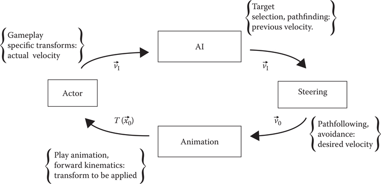
Figure 16.1
A typical game loop.

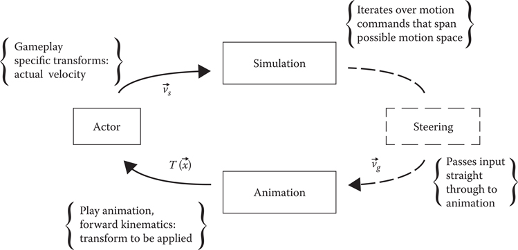
Figure 16.2
The simulation loop.

We expect the game to provide rough estimates of each actor’s motion capabilities, such as its approximate minimum and maximum speed. This range will form the basis of the motion range to explore.

Once the actor has been initialized, a series of movement commands are issued to the actor. It is recommended that the actor be given a deterministic set of movement commands and that each command perform some sampling, so some measure of variance can be calculated, as well as noise can be filtered out in the analysis stages. Having a deterministic set of movement commands helps greatly in catching rare bugs, for example, a float overflow in the animation system.

Each simulation command $C_s$ is a point on an interpolation over a range, such as ${\left(v,\text{θ}\right)}_n\to {\left(0,\text{θ}\right)}_n,$ signifying the exploration of the motion from speed $v$ to stopping, over $n$ intervals between $v$ and $0$with a constant facing $\text{θ}$. The set of simulation commands might differ slightly depending on the animation capabilities of the game, but generally, quantities such as speed, turn motion, and so on should be explored.

A command $C_s$ is considered finished once the measurement has reached a stable output. For example, starting at speed $v$ and wanting to reach speed $v_g$, the command is considered complete once the measured output $v_s$ is stable.

16.3.2  Measurement Output

At the end of every command, the observed motion parameters are logged. Below the quantities measured are described with an attached notation set in Table 16.1.

Table 16.1 Measurement Variables and Notation

Name	Notation	Description
Goal speed	$v_g$	The speed at which the actor should travel
Simulated speed	$v_s$	The speed that the actor actually traveled at
Desired angle	${\text{θ}}_g$	The direction to which the actor should travel
Simulated angle	${\text{θ}}_s$	The direction in which the actor traveled

We declare the rotational speed to be $\partial \text{θ}/\partial t=\dot{\text{θ}}$ for time $t$. The raw measurements are therefore a set of trajectories where each data point $T_i$ on the trajectory is defined as the tuple:

$T_i=(t,\overrightarrow{p},{\text{θ}}_s,{\dot{\text{θ}}}_s,v_s)$

with $\overrightarrow{p}$ as the position on the trajectory. From the trajectories $T_i$, other quantities can then be derived, such as variance of speed and rotation, distance travelled, and so on.

16.4  Building an Accurate Movement Model

Once the measurement phase is complete, the construction of the movement model that accurately describes the actor begins. The following sections will address different parts of an actor’s motion and will give a rough overview of how the model parameters are formed.

16.4.1  Speed

The first constraint to determine is the speed range of an actor, as it will go on to inform the rest of the model construction. Our goal is to find the largest speed range in which the error between the goal speed $v_g$ and the stable simulated speed $v_s$ will not exceed a given minimum error. We determine the valid speed range using only data points where the actor is moving straight forward, that is, with $\dot{\text{θ}}=0$ and at a stable speed $\dot{v}=0$. Figure 16.3 depicts the stable speeds obtained from fixed input speeds in these data (for a dog character). The error in this graph is the deviation between the resulting speed and the goal speed $\text{ε}=|v_g–v_s|/v_s.$ We look for the largest interval of speeds in which $\text{ε}$ does not exceed a fixed bound. Minimum and maximum speed then simply equate to the bounds of this interval.

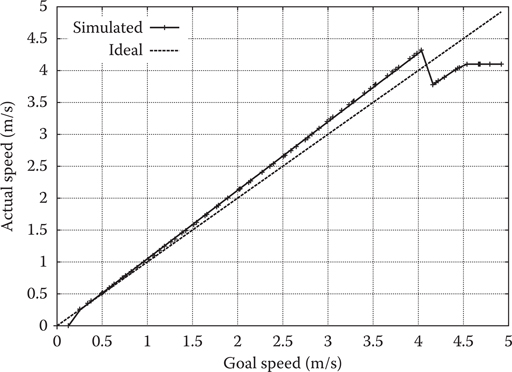
Figure 16.3
Speed measurements.

If no speed range can be determined in this way, or if the speed range is significantly smaller than expected, the simulation is marked as a failure and no model is extracted, such as in Figure 16.3 where a drop in $v_g$ occurs at around 4 m/s.

16.4.2  Stopping

Given the real speed range of the actor, the next part of the motion model can be constructed. As was mentioned in the introduction, stopping on the mark can be a difficult problem both in the real world as in the virtual one. We analyze trajectories where the actor moves at a stable speed in a straight line and stops due to receiving a goal speed of zero.

Since at runtime, we need to answer questions such as when to issue a stopping signal such that an actor will come to a halt at a predetermined goal position; we cast these data as a function of distance mapping onto velocity. In other words, given an available distance $d,$ the function maps to the velocity at which the actor would take exactly a distance of $d$ in order to come to a complete halt. Figure 16.4 shows an example of this curve. It clearly shows data points generated from different stopping animations, that is, stop-from-walking and stop-from-running. After manually analyzing a varied set of characters, we concluded that most data behaved in a piece-wise linear fashion, as shown in Figure 16.4.

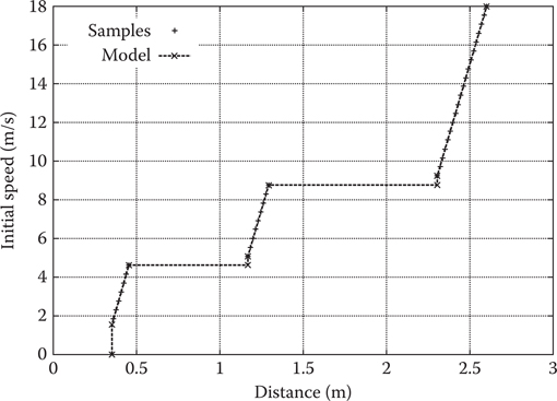
Figure 16.4
Stopping measurements.

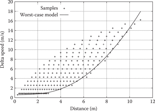
Figure 16.5
Deceleration measurements.

16.4.3  Deceleration

Generalizing from stopping, we arrive at deceleration. Having accurate information about how long it takes to decelerate a given amount of speed allows the actors to fluidly decelerate before taking a turn and to confidently accelerate again afterward.

Figure 16.5 shows a typical result when recording the distance necessary to decelerate by a certain delta speed. Note the large spread for medium delta speeds. This is because the actual relationship depends on the absolute speed, not just the relative speed. The faster an actor travels, the larger a distance is necessary to decelerate by 1 m/s.

Instead of representing the full 3D relationship, we opted to project the data into 2D and use a worst-case estimate:

$\text{Δ}v\left(d\right)=a{d}^2+bd+c\sqrt{d}$

(16.1)

With only three parameters, this is a very compact representation that is easily regressed by using sequential least squares programming. The increase in fidelity when using a 3D representation was deemed too small to warrant the additional memory investment necessary.

16.4.4  Overshoot

Overshoot is a measurement for how much space a character requires to turn. More specifically, it is the distance between the trajectory that a character would follow if it would follow the control input perfectly and the actual trajectory measured after a change in direction has been completed. Figure 16.6 shows the measured distance between ideal and performed trajectory.

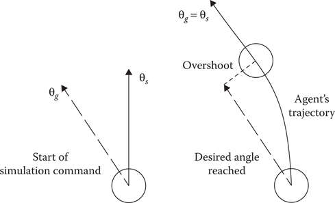
Figure 16.6
Overshoot definition.

This overshoot distance can be represented as a function of velocity and angle.

Figure 16.7 shows the overshoot of a monster in FINAL FANTASY XV. We represent these data as a velocity function over distance and turn angle. The approximation is done as a set of piece-wise linear functions, uniformly distributed over angles between $0°$ and $180°$.

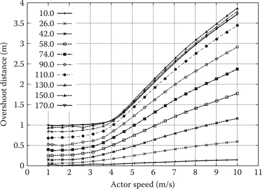
Figure 16.7
Actor speed versus overshoot distance.

16.4.5  Rotation Radius

We record the rotation radius of a character as a function of speed by letting the character run in a circle at a constant linear speed, as shown in Figure 16.8. Thus, we measure the character’s rotational speed. We represent the rotation radius as a piece-wise linear function of speed. Thereby, we assume a constant maximum rotation speed for large proportions of the speed range. At runtime, this information is used to interrupt a movement command early and avoid characters getting stuck on a circular path around their goal position.

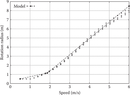
Figure 16.8
Rotation radius measurements.

16.5  Runtime

The extracted motion model is made available to inform steering decisions at runtime.

First and foremost, minimal and maximal speeds are used to limit the range of selectable speeds. The remainder of the data is used to improve control precision. Steering control and animation form a loop in which steering commands are sent to animation, which changes the physical state of the agent, which in turn is observed by steering.

The deceleration function informs the runtime of how much space is needed to achieve a certain negative Δv. Consequently, it is used to calculate the current control speed given a future goal speed. For example, if an agent is supposed to move at 2 m/s at a distance of 3 m, its current speed is capped by the deceleration function to 4 m/s for example. This is used in all cases where a future goal speed is anticipated, such as when charging for an attack and thus arriving with a certain speed at a target or following a path with a tight turn.

Collision avoidance, however, asserts the necessity to stop within a certain distance. The special case of stopping is handled by a stopping function. Deceleration is typically achieved by a combination of a blend and changes to the playback speed. In contrast, stopping typically is achieved by a separate animation altogether. Playing this animation does not fit the simple deceleration model we introduced in Section 16.4.3.

Whenever an agent is required to stop within a certain distance, be it in order to hit its mark, or avoid a collision, an upper limit for the control velocity is looked up in the stopping function. In addition, whenever the current physical velocity of the agent exceeds this limit, the control velocity is immediately pulled down to zero, thereby triggering a transition to a stopping animation. In order to avoid accidentally triggering this stopping maneuver due to noisy velocity measurements, the maximum control velocity is actually capped at 95% of this limit.

The overshoot function is used to calculate the maximum speed while taking a turn and when anticipating a future turn in a path currently followed. In addition, for characters without a turn-in-place animation, such as some larger monsters, it is also used to judge whether to turn left or right when aligning with a path. In case of an anticipated turn, an upper bound of future speed is simply a look up using the sine of the anticipated turn angle; the resulting velocity then serves as an input for the deceleration function to obtain an upper bound for the control speed as described above. In FINAL FANTASY XV, path information is imperfect, meaning that a path may only be part of the surrounding free space. Moreover, the path does not take moving obstacles into account. Thus, for immediate turns, both due to path following and due to collision avoidance, the available distance as given by collision avoidance sampling is used to look up a limit to the control speed in the overshoot function.

Finally, the rotation function is used to avoid circling around a target indefinitely by increasing the arrival radius, given an actor’s current physical velocity and angle to its target.

16.6  Pipeline

All of this work can be wrapped up in a nice little continuous integration loop, as can be seen in Figure 16.9, containing the following steps:

1.  Create a valid movement model for steering.

2.  Provide the developers a view for an actor’s movement model for the whole period of development.

3.  Alert the developer when there is a problematic movement model that needs addressing.

Due to the fact that the simulation of an actor takes more time than to build the animation data per actor, the pipeline structure tries to reduce the lag as much as possible by running constantly. The choice of the next actor to simulate is made by a simple heuristic of the time since last simulation and whether the actor has been just added to the repository. Failures are logged to a database, and stakeholders are automatically notified.

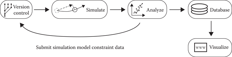
Figure 16.9
Continuous simulation pipeline.

16.7  Scaling Up

There are two scale issues to take into account when building the simulation pipeline.

16.7.1  Size and Playback

A game might want to scale the size of actors and expect the motion constraint model to still apply. Similarly, the animation playback rate might vary on a frame-to-frame basis. Both factors must be applied to the motion model and, depending on the different parts in the model, both size and/or time scales must be applied. As an example, the deceleration function (Equation 16.1 in Section 16.4.3) with respect to size scaling $u$ and playback rate scale $p$ becomes:

$\text{Δ}v\left(d,u,p\right)=p\left(\frac{a{d}^2}{u}+bd+c\sqrt{ud}\right)$

The rest of the overall model is either multiplied by $u,$ $p,$ or both.

16.7.2  Content

When the need arises to scale up the number of entities via the use of prefabs, the simulation pipeline does not suffer as much from the time delay between authoring data and exporting constraints. However, there is still a possibility that the prefabs have an element in either some part of their unique-data setup or in code that will differentiate their motion, and there is no easy way to test this without simulating all users of the prefab and doing a similarity test between the results.

16.8  Benefits

The biggest benefit of this methodology is how well it scales to differences in characters and changes to the data and code throughout the development cycle. Precision is also increased with this methodology. As an example, the stopping distance is normally the distance of some “to-stop” animation plus whatever may be done to the animation in the runtime. This overall distance can be hard to parameterize at the authoring time, but the simulation can easily extract the worst case from the observed movement.

Issues, such as a nonmonotonic speed function, can be easily identified from a graph, instead of through loading the game. This is seen in an example of a FINAL FANTASY XV cat speed graph found in Figure 16.10.

When comparing the speed graphs of cats (Figure 16.10) and dogs (Figure 16.3), it is clear from the simulated data that cats are indeed more independent than dogs with respect to speed, at least in FINAL FANTASY XV.

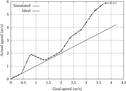
Figure 16.10
Speed measurements of a cat.

16.9  Conclusion

We have presented a way of significantly decoupling dependencies between AI and animation. This approach treats animation as the dominant party in this relationship of motion and shows a way of gaining benefit from such an approach.

Although significant work was invested in setting up and maintaining the pipeline, the work needed to identify and fix issues has dramatically decreased. Typically, it amounts to analyzing graphs on a web server and determining from there what the fault is. Common bugs include the gait being exported from the raw animation, so the actor does not have a fixed acceleration or a genuine code bug that has been introduced, which can be found by looking at the graphs by date and revision to determine what revision introduced the code bug.

Overall, the usage of simulations to improve steering control of an animation-driven agent has proved to be a success. It is not particularly expensive at runtime, as the models are mostly sets of piece wise linear functions and one nonlinear function. Furthermore, scaling of size, playback rate, or both are easily supported.

References

Ciupinski, J. 2013. Animation-driven locomotion with locomotion planning. In Game AI Pro: Collected Wisdom of Game AI Professionals, ed. S. Rabin. Natick, MA: A. K. Peters, Ltd, pp. 325–334.

Gregory, J. 2009. Game Engine Architecture. Wellesley, MA: A. K. Peters, Ltd.