
The AI of Driver San Francisco
Driver San Francisco was an open-world driving game set in a fictionalized version of the city of San Francisco. The game’s version of the city was very large, and in some areas had very dense traffic.
The player was given different missions that involved navigating through traffic at high speeds interacting with other mission-critical NPC vehicles, which also had to move quickly through the traffic. NPC vehicles might be chasing another vehicle, evading a vehicle, racing around a set course or trying to get to a particular point in the city. Also, at any point, the player could switch vehicles and start controlling any other car in the city; when this happened, it was the job of the AI to take over control of the player’s vehicle, continue driving, and try to achieve the player’s mission objective.
An important part of the game design was to produce dramatic, cinematic car chase sequences. Due to this, the AI-controlled vehicles as well as the player vehicle were often the centers of attention, being closely watched by the game camera. To create the most impressive visuals, it was a requirement that the AI code could control a vehicle simulated by the same system that was used for the player vehicle. We were not allowed to cheat by giving the AI vehicles more power or tighter grip between the tires and the road. We also had to perform at a level that was similar to the best human players, so the cars had to be capable of coming close to the limits of friction when cornering, without pushing too far and skidding out of control.
The game was designed to run at 60 frames per second. This put a significant restriction on the amount of work we could do in any single frame. For this reason, the AI system was designed to be asynchronous and multithreaded. Individual tasks to update the state of a particular AI were designed to run independently and to update the state of the AI when the task was finished. Even if the task was finished after several frames, the AI would be able to continue intelligently while waiting for the result.
Planning a path for the AI vehicles in this environment posed several problems:
• The vehicles’ main interactions were with other vehicles, so the path planning had to deal with moving obstacles. This meant that we had to look ahead in time as well as space and plan to find gaps in traffic that would exist at the time we got to them.
• Valid paths for vehicles must take into account parameters of the physical vehicle simulation, such as acceleration, turn rates, and tire grip if they are to be feasible for a vehicle to drive.
Classical path planning algorithms such as A* work well for static environments of limited dimension, but trying to search through a state space including time, velocity, and orientation would be impractical.
In this chapter, we present the path planning solution Driver San Francisco used: a three-tier path optimization approach that provided locally optimal paths. The three stages of the process—route finding, mid-level path planning, and low-level path optimization—will be detailed in the subsequent sections.
Driver San Francisco had two distinct types of AI to control his or her vehicles: Civilian Traffic AI and Active Life AI. Civilian vehicles were part of a deterministic traffic system that simply moved vehicles around a set of looping splines throughout the city. Each spline had been defined to ensure that it did not interact with any other spline. Each civilian vehicle would follow a point around the spline, knowing that there was no chance of colliding with other civilian vehicles. Nontraffic vehicles were controlled by the more complex Active Life AI system. These vehicles perform much more complex actions than simply blending in with traffic, such as racing, chasing, or escaping from other vehicles. The Active Life AI system performed much more complex path generation.
Driver San Francisco’s most important gameplay mechanic, shift, allowed players to switch cars at any point. When the player activated shift, the vehicle the player left was taken over by an Active Life AI, which would start running the appropriate behavior to replace the player. For example, if the player shifted out of a cop car chasing a suspect, the AI would give a “chase target” behavior to the cop car, which would continue what the player was doing before the switch. If the player had been driving a civilian vehicle with no particular objective, the AI would select the closest free slot on the traffic splines and try to rejoin traffic; as soon as this happened, the driver was downgraded to a regular civilian vehicle.
17.2.1 Vehicle Paths
As any car could transition from civilian to Active Life and vice-versa at any moment, it was important to keep an unified system to define what vehicles were trying to do, so each one owned a vehicle path. These paths represented the predicted movement of the vehicle for the next couple of seconds, and the AI system was constantly updating them—actually, path updating happened approximately every second. Paths were updated appending new segments at their end before they were completely used. So, from the vehicle’s perspective, the path was continuous. Updating paths this way allowed us to run costly calculations in parallel over multiple frames. Even the player’s vehicle had a path!
The way vehicle paths were generated depended on the system that was controlling them. For player vehicles, physics and dead reckoning generated this path; traffic splines generated paths for civilians. For Active Life AIs, we used different levels of detail, based on range to the AI. We had three levels of detail (LODs):
• AIs using the lowest level of detail generated their paths using only their route information. A route, as we will talk about later, is a list of roads that can take us from point A to B. These roads are defined as splines, and these splines are connected by junction pieces. Routes were basically very long splines. Low-LOD vehicle paths were a portion of the route’s spline with an offset to simulate that they were driving in a certain lane on the road.
• The next level of detail used mid-level paths to generate vehicle paths. A mid-level path is a first approximation of a good path for a vehicle. It uses the route information plus some extra details, such as lane information (we prefer maintaining our current lane if possible), some rough dynamic obstacle avoidance, and some speed limit data. Mid-level path generation is described in detail in a subsequent section.
• Finally, the highest level of detail was used for vehicles around the player that were in camera and needed to be fully simulated and as polished as possible. They used the full three-tier path generation (route finding, mid-level path planning, and low-level path optimization).
The vehicle paths also supported another significant optimization in the game’s simulation code. The large number of vehicles being simulated in the world at any one time would be very costly in terms of physics and vehicle handling. For this reason, there was a system of simulation level of detail acting at the same time as, but independently of the AI LOD. When vehicles were close to the player, they would be fully simulated by the physics and handling system, and they would follow their paths using the AI path-following system to calculate driving input into the handling system. When vehicles were distant from the player, they could be removed from the physics engine and vehicle-handling code, and simply placed at the position defined by their path for that particular time.
17.2.2 Driver Personalities
In the game, AIs had different goals, but also different driving styles or personalities. AIs had a set of different traits that defined their characters. Some examples of these traits were:
• Likeliness to drive in the oncoming traffic.
• Likeliness to drive on sidewalks.
• Preferred driving speed.
• How desirable highways, alleyways, or dirt roads were?
• How strongly hitting other vehicles should be avoided?
Personality traits affected every stage of the path planning, as we will see in later sections.
Our virtual San Francisco was, in the eyes of the AI, a network of interconnected roads. For each of these roads, the game exposed the following information, as shown in Figure 17.1:
• A spline that represents the road.
• Each road had a start and an end extremity. For each extremity, we had:
• A list of roads that were connected to the extremity.
• Cross-section information: This defines the number of lanes at the extremity, as well as the width and the type of each of these lanes.
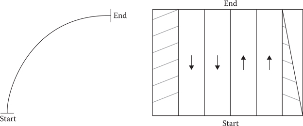
Figure 17.1
An example road spline with its cross section information.
In the example, our road has two directions. We call the lanes that travel from the start to the end extremity as “with traffic” lanes, and the ones traveling in the opposite direction are called “oncoming.” The example road presents two “with traffic” and two “oncoming” lanes; it also has a sidewalk on the oncoming side (the left-most lane on the cross section) and a sidewalk on the right side of the road that disappears at the end of the spline.
The path generation process for Active Life AIs started by selecting the roads that these vehicles would use to reach their destination. The goal was to generate a list of connected roads, a route, which allowed cars to drive to their destination. For this, we used the connectivity information in the road network.
Depending on the goal or behavior of a vehicle, we used one of the following two methods to generate a route:
• A traditional A* search on the road network was used when we knew what our destination road was.
• A dynamic, adaptive route generator was used by the AI when its objective was to get away from a pursuer. For more details on this system, readers can refer to Ocio (2012).
Due to the size of the map and the strict performance requirements the AI systems had to meet (Driver San Francisco runs at 60 FPS on Xbox 360, PS3 and PC), we split the map in three different areas, which are connected by bridges, and used a hierarchical A* solution. If two points, A and B, were in different areas, we would first find a path to the closest bridge that connected both areas, and then find a path from the bridge to position B on the second area.
The path planning system itself imposed extra requirements. For instance, we always needed to have “enough road length” ahead of our vehicle, so sometimes an artificial node was appended at the end of the route. This was very often the case when an AI was following another vehicle, and both cars were pretty close to each other. This extra road allowed vehicles to predict where they should be moving to next and helped them maintain their speed. This will be explained in the following sections. During a high-speed chase, approaching junctions required a constant reevaluation of the intentions of the vehicle being chased. The goal was to predict which way the chased car was trying to go. We achieved this by making use of our simplified physics model that provided us with a good estimation of what a car was capable of doing based on its current state and capabilities. Figure 17.2 depicts the problem.
Route finding was also affected by the personality of the driver. The cost of exploring nodes varied based on the specific traits of the AI, and this could produce very different results. For example, civilian-like drivers could follow longer but safer routes to try and avoid a dirt road, whereas a racer would not care. Finally, AIs would, in some situations, try to avoid specific roads. For instance, a getaway driver would try to not use roads with cops.
Driver San Francisco’s path planning solution did not look for optimal paths, as a more traditional A*-based approach would normally do. Instead, we were trying to generate locally optimal paths by optimizing some promising coarser options that we called mid-level paths. Mid-level path planning was the second stage of our three-tier process that happened after a route had been calculated.
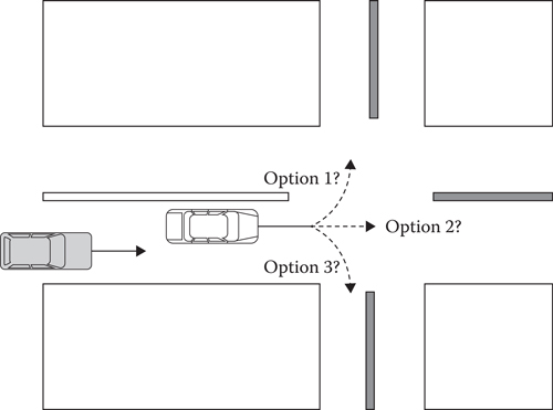
Figure 17.2
When chasing another vehicle, our AIs needed to decide which road the chased car was going to take at every intersection.
The route was defined in terms of the splines describing the center lines of the roads we wanted to follow, but it contained no information about which road lane we should drive down. The mid-level path allowed us to specify where on the road the vehicle should drive. The mid-level path was generated by searching for a path between a set of possible path nodes spread out in a grid over the road in front of the vehicle. The search space began at the current position of the vehicle and extended forward down the road far enough that the path would be valid for several seconds. The search space would typically be about 100 m in length. We placed sets of nodes at regular intervals over this part of the spline. With regard to width, one node was placed in each traffic lane. We show an example search space in Figure 17.3.
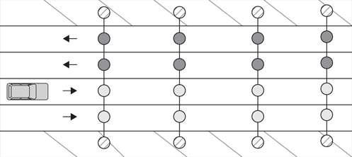
Figure 17.3
Node sets placed every few meters along the roads in the route constitute our search space for the midlevel path planning.
Once the search space was defined, we generated all the possible paths from the vehicle to each node on the last set, scoring them, and then selecting the five best options, which became the seeds for the optimizer. Evaluating a path meant giving each node used a numeric value; the final cost would be the sum of all the individual values. The game used costs for paths, which meant the higher the number, the less ideal the path was. The criteria used to generate these costs were:
• Nodes near dynamic obstacles (i.e., other vehicles) were given some penalty; if the obstacle was static (e.g., a building), the node could not be used.
• We always preferred driving in a straight line, so part of the score came from the angle difference between the vehicle’s facing vector and the path segment.
• Depending on the driver AI’s personality, some nodes could be more favorable. For example, a car trying to obey traffic rules will receive big penalties from driving on sidewalks or in the oncoming lane, whereas a reckless driver would not differentiate between lane types.
Figure 17.4 shows a couple of example mid-level paths and their costs.
In the example, the cost calculation has been simplified for this chapter, but the essence of the process remains. Moving in a straight line costs 1 unit and switching lanes costs 2 units. Driving close to another car costs an additional point, so does driving in the oncoming lane. With these rules, we calculated a cost of 5 for the first path and 11 for the second one.
Although in Figure 17.4, we treated other vehicles as static when we calculated the cost of driving next to an obstacle, in the real game, these calculations were made taking into account current vehicle speeds and predicting the positions of the obstacles (by accessing their vehicle paths). So path 2 could potentially have been scored even higher in a couple of locations. For example, the first node, which got a cost of 4, could have produced a bigger cost if the car driving in the opposite direction was moving. Path 1 could have even just been a completely straight line, if the vehicles we are trying to avoid in the example were moving fast enough, so they were not real obstacles for our AI!
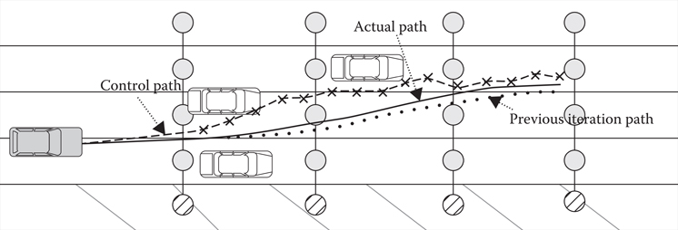
Figure 17.4
Two possible midlevel paths found for the given search space; path 1 has a lower cost, so it would be the preferred option.
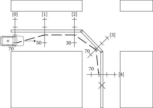
Figure 17.5
Midlevel paths contained information about the maximum speed the vehicle could travel at each of their nodes.
Another piece of information we could get out of mid-level was speed information and, particularly, speed limitations, or how fast a corner can be taken without overshooting. Starting from the last node set backward, we calculated the maximum speed at certain nodes based on the angle that the path turned through at that node. This speed was then propagated backward down the path based on the maximum acceleration/deceleration, so the path contained some information the vehicle could use to start slowing down before taking a corner. Figure 17.5 shows an example mid-level path with speed limits.
In the example, calculations would start at node set 4. The maximum speed at that node is the maximum desired speed for our vehicle (let us use 70 mph for this). Traveling from node 3 to node 4 is almost a straight line, so the vehicle can travel at maximum speed. However, moving from node 2 will require a sharp turn. Let us say that, by using the actual capabilities of our car, we determined the maximum speed at that point should be 30 mph. Now, we need to propagate this backward, so node 1 knows the maximum speed at the next node set is 30. Based on how fast our vehicle can decelerate, the new speed at node 1 is 50 mph. We do the same thing for the very first node, and we have our speeds calculated. Path speeds also took part in the path cost calculation; we tried to favor those paths that took us to the last set of nodes faster than others.
Mid-level paths represented a reasonable approximation of a path that could be driven by a vehicle, but this was not good enough for our needs. Although the velocity of the path has been calculated with an idea of the capabilities of the vehicle, the turns have no representation of the momentum of the vehicle or the limits of friction at the wheels. These problems are resolved by the low-level path optimizer.
The low-level optimizer uses a simplified model of the physics of the vehicle, controlled by an AI path-following module, to refine the path provided by the mid-level into a form that a vehicle could actually drive. When the constraints on the motion of the vehicle are applied to the mid-level path, it is likely to reduce the quality of the path—perhaps the vehicle will hit other cars or skid out of control on a tight corner. These problems are fixed by an iterative path optimization process.
To choose a good path, it was necessary to have a method of identifying the quality of a particular path. This was done by creating a scoring system for paths that could take a trajectory through the world and assign it a single score representing the desirability of the path. Good paths should move through the world making forward progress toward our goal as close as possible to a desired speed while avoiding collisions with other objects. The aim of the optimization process is to find a path with the best possible score.
The environment through which the vehicles were moving is complex, with both static and dynamic obstacles to avoid, and a range of different target locations that could be considered to be making progress toward a final goal. To simplify the work of the optimizer, the environment is initially processed into a single data structure representing where we want the vehicle to move. This structure is a potential field, in which every location in the area around the vehicle is assigned a “potential” value. Low-potential areas are where we want the vehicle to be, and high-potential areas are where we want the vehicle to move from. Good paths can then be found by following the gradient of the potential field downward toward our goal.
The various different systems that came together to form the low-level path optimizer are described in the following sections.
17.6.1 Search Area
Before the optimizer could start generating paths, it needed to prepare data to use during its calculations. The first piece of data we prepared was a small chunk of the world where the path planning process would take place, the search area.
A rectangle was used to delimit the search area. This rectangle was wide enough to encompass the widest road in the network, and it was long enough to allow the vehicle to travel at full speed for a couple of seconds (remember mid-level paths were generated for this length). The area was almost centered on the AI vehicle, but not quite; while the car was indeed centered horizontally, it was placed about ¼ along the rectangle’s length. Also, the area was not axis aligned. Instead, we would use the vehicle’s route to select a position in the future and align the rectangle toward this point. Figure 17.6 shows an example rectangle.
After the rectangle was positioned, we detected the edges of the roads and used them to calculate inaccessible areas. Vehicles in Driver San Francisco were only able to drive on roads and some special open areas, designer-placed zones attached to a road spline that we wanted to consider as a drivable area. Likewise, we had closed areas or zones that we wanted to block, such as a static obstacle. Figure 17.7 shows the previous search zone, now annotated with some example areas.
In this example, the lower left building was cut by an open area, and a road separator (closed area) was added to the first road in the route.
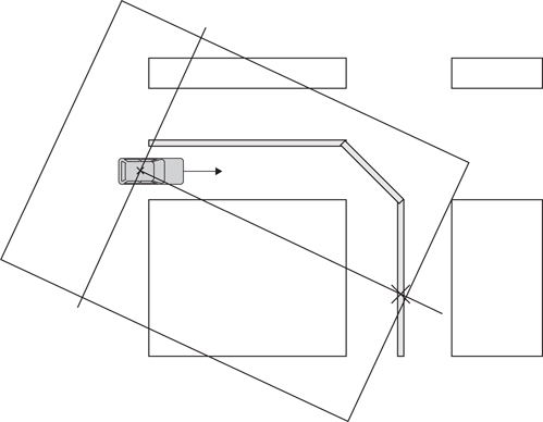
Figure 17.6
The search area is a rectangular zone that encompasses the surroundings of the AI vehicle.
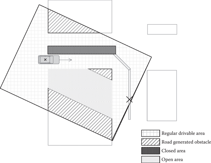
Figure 17.7
The search area’s static obstacles were calculated from the road information and from some special areas placed by designers on the map to open or close certain zones.
The search area was used to define the limits within which we calculated a potential field, where the potential of a particular area represents the desirability of that location for our AI. Movements through the potential field toward our target should always result in a lowering of the potential value. Areas that were inaccessible because of static or dynamic obstacles needed to have high potential values. As the path planning algorithm was trying to find a path that was valid for several seconds into the future, and other vehicles could move a significant distance during the time that the path was valid, it was important that we could represent the movement of obstacles within the potential field. For this reason, we calculated both a static potential field and a dynamic potential field. By querying the static potential field for a particular location, querying the dynamic potential field at the same location for a particular time, and then summing the results, we could find the potential for a location at a particular time. Similarly, we could find the potential gradient at a location at a particular time by summing the potential gradient value from both fields.
17.6.2 Static Potential Field
With the search area defined, the next data calculated were a static potential field. This was used to help us define how movement should flow—in what direction while avoiding obstacles. It worked almost as water flowing down a river. This potential field was created using the fast marching method (Sethian 1996). The search area triangle was split into a grid, so we could do discrete calculations. We set a row of goal positions at the end part of the search area rectangle and calculated the values for each cell in the grid.
For the algorithm, we needed to define the propagation speed at each cell, and this came mainly from the type of lane below the cell’s center position and the personality of the AI driver. For a civilian driver, for example, a cell on the oncoming late should be costlier to use, which means the gradient of the field on those cells will be pointing away from them. Figure 17.8 shows what the field’s gradient would look like in our example.
In this example, we set two goal cells for the potential field. With a civilian personality, oncoming lanes should normally be avoided, and sidewalks should be avoided at all costs. This produced a nice gradient that helps navigate toward the goals. If we dropped a ball on any cell and move it following the arrows, we will end up at the objective cell.
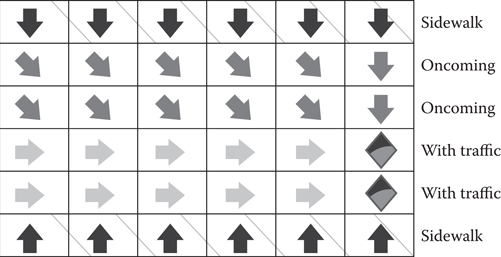
Figure 17.8
The search area was split into cells, and a potential field was generated to show how movement should flow to avoid static obstacles.
17.6.3 Dynamic Potential Field
AIs in Driver San Francisco had to deal with static obstacles but mostly with dynamic, moving ones. Although the static potential field was necessary to avoid walls, we needed a way to produce some extra forces to avoid surrounding vehicles. The approach taken in Driver San Francisco was to apply these forces as an extra layer on top of the static field.
The dynamic potential field could be queried at any point for any particular time. If we visualized it overtime, we were able to see forces produced around vehicles, pushing things out of the obstacle. Clusters of vehicles could produce gaps between them or forces to go around the whole cluster, depending on how far apart the different vehicles were. Figure 17.9 shows an example.
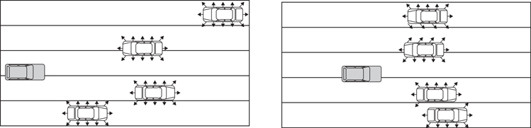
Figure 17.9
The dynamic potential field dealt with moving obstacles, generating forces around them so they could be avoided.
17.6.4 Simple Physics Model
The vehicle motion in the game was modeled using a complex physics engine with 3D motion, and collisions between dynamics and with the world. Vehicle dynamics were calculated using a wheel collision system and modeling of the suspension extension, which gave information about tire contacts with the world feeding into a model of tire friction. The wheels were powered by a model of a vehicle drive train applying a torque to the wheels.
This model was computationally expensive, but we needed to get some information about what constraints this model applied to the motion of the vehicle into our path planning algorithm, in order to create paths that the vehicle was capable of driving.
The fundamental aspects of vehicle behavior come from the torque applied by the engine and the tire forces on road, and this part of the vehicle simulation can be calculated relatively quickly. We implemented a simple 2D physics simulation for a single vehicle, driven by the same inputs as the game vehicle. This simulation shared the engine and drive-train model and the tire friction calculations from our main game vehicle-handling code but made simplifying assumptions about how the orientation of the vehicle changed as it was driving. Parameters of the handling model were used to ensure the simulation of vehicle was as close to the full game simulation as possible. The results of collisions were not modeled accurately; this was not a significant problem as the aim of the optimization process was to avoid collisions, so any paths that lead to collisions were likely to be rejected by the optimization process.
17.6.5 AI Path Following
To control the vehicle in the simple physics simulation, a simple AI path-following module was used. This module was exactly the same as the AI that was used to follow paths in the real game. The AI was fed with information about the current dynamic state of the vehicle and details of the path it was expected to follow. The module calculated controller input based on these data that were sent to the vehicle simulation. The action of the AI in any frame is based on the desired position and orientation of the vehicle, as defined in the path it is following, at a time in the future.
Internally, the AI used a simple finite-state machine to define the type of maneuver that was being attempted. Each state had some heuristics that allowed the control values to be calculated based on the differences between the current heading and velocity and the target position and orientation of the vehicle.
17.6.6 Simulating and Scoring a Path
The physics simulation and AI code could be used together to simulate the progress of a vehicle following a path. The physics simulation could be initialized with the current dynamic state of the vehicle, and then it could be stepped forward in time using the AI module to generate control inputs designed to follow a particular control path.
The output of this simulation was the position and orientation of the vehicle at each step of the simulation. We will refer to this series of position/orientation pairs as an actual path for a vehicle. This path generated for a particular control path is the trajectory we would expect the vehicle to follow if the control path was used to control the full game simulation representation of the vehicle. It is worth noting that we expect the actual path to deviate from the control path to some extent, but that the deviation should be small if the control path represents a reasonable path for the vehicle to take, given its handling capabilities.
The score for a particular control path is calculated by considering the actual path that the vehicle follows when given that control path. The total score is calculated by summing a score for the movement of the vehicle at each step of the physics simulation. In our case, we chose to assign low scores for desirable motion and high scores for undesirable motion, which leads to us trying to select the path that has the lowest total score. The main aim of the scoring system was to promote paths that moved toward our goal positions, avoided collisions, and kept the speed of the vehicle close to a desired speed. To promote these aims, the score for a particular frame of movement was calculated by summing three different terms:
• Term 1 was calculated from the direction of the movement vector of the vehicle over that frame, compared with the gradient of the potential field at the vehicle’s location and the time of the frame. The value of the dot product between the two vectors was scaled and offset to add a penalty to movements that went toward higher potential.
• Term 2 was calculated by considering the current speed of the vehicle and the desired speed. The absolute value of any difference between the two was added to the score.
• Term 3 was calculated based on collisions. If the physics engine had found any collisions for the vehicle on that frame, a large penalty was added to the score.
The three terms were scaled by factors we arrived at empirically to give the best results.
17.6.7 Optimizing a Path
A single mid-level path can be converted to a path that is suitable for the capabilities of the vehicle that has to drive it. Initially, the mid-level path is converted into control path by sampling points from it at regular time intervals, corresponding to the frame times for the simplified vehicle simulation. This control path is then scored by passing it through the simplified simulation system as described in Section 17.6.6, which generates an actual path for the vehicle. This is shown in Figure 17.10.
This actual path can then be compared with the potential field and used to generate an optimized control path that we expect to have a lower score. First, the actual path is converted to a control path by using the positions of the vehicle at each frame to represent the positions in the control path. These positions are then adjusted based on the gradient of the potential field at those points. This process will push the path away from areas of high potential—that is, obstacles and parts of the world where we would prefer the vehicle not to drive. Figure 17.11 shows the results of this first iteration of the optimization process.
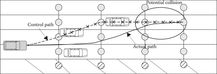
Figure 17.10
The first control path is created from the midlevel path we used as a seed and can still present problems, such as potential collisions.
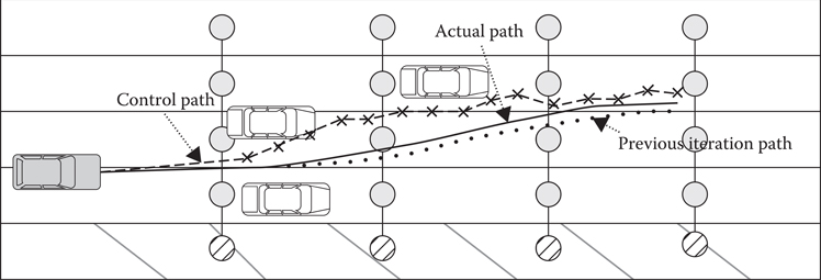
Figure 17.11
Vehicle positions along the first actual path are modified by the potential field; we use this as our second control path, which generates an optimized version of the original actual path.
This optimized control path is then ready for evaluation by the scoring algorithm and can be optimized again in an iterative process while the score continues to decline. The paths that we are dealing with only last for a few seconds, and over that time, the motion of the vehicle is initially dominated by its momentum. The control input can only have a limited effect on the trajectory of the vehicle through the world. Due to this, we found that three or four iterations of the optimization loop were enough to approach a local minimum in scoring for a particular mid-level path starting point.
17.6.8 Selecting the Best Path
The optimization process begins with a set of five potential paths from the mid-level planner and ends up with a single best path that is well suited to the capabilities of the vehicle that is expected to follow the path. Each mid-level path was optimized in turn, iterating until it reached a local minimum of score. The path that leads to the lowest score overall is selected as the final path and returned to the vehicle to be used for the next few seconds.
Driver San Francisco’s AI used state-of-the-art driving AI techniques that allowed the game to run a simulation with thousands of vehicles that could navigate the game’s version of the city with a very high level of quality, as our path generation and following used the same physics model as any player-driven vehicle. The system was composed of multiple levels of detail, each of which updated vehicle paths only when required to do so. This allowed the updates to be spread asynchronously across many threads and many frames, meaning the game could run smoothly at 60 FPS. Path optimization allowed the system to deal efficiently with a world composed of highly dynamic obstacles, a world which would have been too costly to analyse using more traditional A*-based searching.
Ocio, S. 2012. Adapting AI behaviors to players in driver San Francisco: Hinted-execution behavior trees. In Proceedings of the Eighth AAAI Conference on Artificial Intelligence and Interactive Digital Entertainment (AIIDE 12), October 10–12, 2012, Stanford, CA.
Sethian, J. A. 1996. A fast marching level set method for monotonically advancing fronts. Proceedings of the National Academy of Sciences 93(4), 1591–1595.