
How They Really Work
19.3 Examining RVO’s Guarantees
19.4 States, Solutions, and Sidedness
19.7 Gradient Methods Revisited
19.9 Putting It All Together: How to Develop a Practical Collision Avoidance System
The reciprocal velocity obstacles (RVO) algorithm and its descendants, such as hybrid reciprocal velocity obstacles (HRVO) and optimal reciprocal collision avoidance (ORCA), have in recent years become the standard for collision avoidance in video games. That is a remarkable achievement: Game AI does not readily adopt new techniques so quickly or broadly, particularly ones pulled straight from academic literature. But RVO addresses a problem that previously had no broadly acceptable solution. Moreover, it is easy to understand (because of its simple geometric reasoning), easy to learn (because its creators eschewed the traditional opaqueness of academic writing, and wrote about it clearly and well), and easy to implement (because those same creators made reference source code available for free). Velocity obstacle methods, at least for the moment, are the deserving rulers of the kingdom of collision avoidance.
Which is why it is a little ironic that very few people actually understand how VO methods work. Not how the papers and tutorials and videos describe them as working, but how they really work. It’s a lot weirder, more complicated, and cooler than you suppose.
There are four stages to really getting RVO:
1. Understanding the assumptions that RVO makes, and the guarantees it provides.
2. Realizing that those assumptions and those guarantees are, in practice, constantly violated.
3. Figuring out why, then, RVO still seems to work.
4. Tweaking it to work even better.
In the remainder of this chapter, we will take you through these stages. Our goal is not to present you with a perfect collision avoidance system but to walk you through the nuances of VO methods and to help you iteratively develop a collision avoidance system that works well for your game. First, though, a brief history of RVO, and VO methods in general. We promise it’s important.
The velocity obstacle method originally targeted mobile robots—that is to say, real physical robots in the real world, moving around without hitting each other. Compared to previous approaches to robot steering, velocity obstacles were intended to be:
• Decentralized, with each robot making its own decisions rather than all robots being slaved to a central controller.
• Independent, with decisions based solely on each robot’s observation of other robots’ positions and velocities.
These features are not of much use to game developers, but they are important to understanding the strengths and weaknesses of VO methods. VO agents do not explicitly communicate or coordinate with each other. Cooperation between them is an emergent effect of their observations, decisions, and actions over time. VO methods spare us the morass that is multiagent planning, focusing on the behavior of individual agents. But the lack of coordination means that agents can make mistakes when predicting what other agents are going to do, thus failing to cooperate properly.
The original VO method was hilariously prone to such failures, with two agents almost guaranteed to start oscillating back and forth when they encountered each other, as in Figure 19.1. Each expected the other to be a mindless blob traveling at a constant velocity, and each was repeatedly surprised when the other instead changed direction and ruined its plan.
19.2.1 Introducing RVO
Those oscillations motivated the design of RVO (van den Berg et al. 2008). The idea was to come up with a decision process for the agent, which assumed that the other agent was also using that decision process. Each agent would move only halfway out of the way of a collision, anticipating that the other agent would do its part as well by moving halfway in the other direction. The paper proved that this would eliminate incorrect predictions, and set agents on optimal noncolliding paths in a single step once they came into view. This is shown in Figure 19.2.
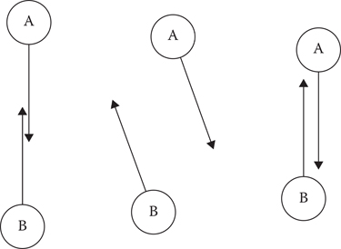
Figure 19.1
The original velocity obstacles method causes oscillation between two agents attempting to avoid each other.
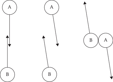
Figure 19.2
The reciprocal velocity obstacles resolve an upcoming collision between two agents in a single frame, putting them on optimal noncolliding trajectories.
19.3 Examining RVO’s Guarantees
The proof of collision-free movement only holds for a world containing two agents (and no obstacles). With only two agents, each one is free to choose the perfect reciprocating velocity, without having to also dodge something else. Moreover, with nothing else in the world, each agent can assume that the current velocity of the other agent is also their preferred velocity.
Let us throw a third agent into the mix and see what happens in Figure 19.3. A and B are moving south side-by-side, when they see C coming toward them. A dodges a bit west, assuming that C will dodge a bit east. B dodges a bit east, assuming that C will dodge a bit west. Obviously C cannot do both of these. In fact it does neither, instead dodging west in order to pass to the west of both A and B. (It would be equally valid for C to dodge east instead, but let’s say it breaks ties by going west.)
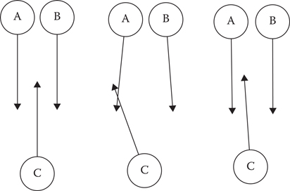
Figure 19.3
Three RVO agents attempting to resolve an upcoming collision.
All three agents are unhappy now. A and C are on a collision course, having both dodged west. B is not going to hit anything, but it has dodged for no good reason, straying from its preferred velocity. For C, it makes the most sense to move to a nearly northward trajectory; its deviation back east, it thinks, will be reciprocated by A deviating west, and even after B’s reciprocation will graze by B. A decides to return to a due south trajectory, which it likes doing better and which it expects C to reciprocate by going even further west than he or she was already. B also returns to due south, reasoning that C is going so far west now that B does not have to worry about a collision.
In short, after two frames, we are back to the original problem. The oscillation that RVO solved for two agents still occurs for three. RVO, in other words, is not guaranteed to avoid collisions in situations such as the above because of an inconsistent view of possible velocities and preferred velocities between agents.
Except … it does avoid collisions. Set up that situation in a real RVO implementation, and C will get past A and B just fine. We have seen that the noncollision guarantee does not hold here, so what is really going on?
Well, after two frames, we aren’t really back to the original problem. Over the two frames, A and B have moved slightly apart from each other. C has moved slightly west and is now traveling slightly west of north. In future frames, these displacements become more pronounced affecting later decisions. While there is a great deal of “flickering” going on with the velocities initially, the three eventually manage to cooperate.
In fact, you could argue that that’s what real cooperation should look like, with each agent not only guessing each other’s plans but reacting when those guesses don’t work out. Eventually the three make simultaneous decisions that are entirely compatible, and then they stick to them until they are safely past.
So reciprocation—perfect avoidance through perfect prediction—has failed. Has RVO, then, gained us anything over original VO? As it turns out, yes. Run the scenario with VO avoidance, and the three will oscillate for much longer. It is easy to construct scenarios where RVO will avoid collisions and VO will not. There’s something more to RVO, beyond the possibility of getting it right the first time.
In Figure 19.4, let’s look at a scenario where A is going south toward B. But, let’s also say that B is malfunctioning, and at a standstill rather than performing proper avoidance.
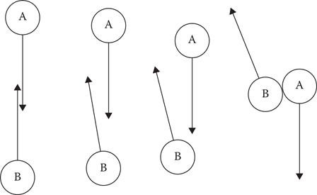
Figure 19.4
An RVO agent steers around a malfunctioning agent.
This is a perfect scenario for A to be using VO, and you might expect RVO to fail entirely, expecting a reciprocation that never comes. Surprisingly, though, RVO still works pretty well! On the first frame, A only dodges half as much as it should… but on the second frame, seeing that a collision is still imminent, dodges half of the remaining half… and then a half of that on the third frame… and so on, asymptotically avoiding the collision. (More or less.) A really expected B to dodge, but when it did not, A could deal with that too.
The magic in RVO, then, is that it strikes a balance between eager collision avoidance and a cagey wait-and-see attitude. An RVO agent faced with a collision dodges some, but not all, of the way. It is less likely than VO to dodge too much, overshooting the optimal velocity and requiring corrections. Moreover, if it has dodged too little, it’s still set up to make up the difference on future frames. This magic is not unique to RVO: so-called gradient methods, such as the gradient descent algorithm for finding minima of functions, and similar techniques, use a multiplier to avoid overshooting the goal.
19.4 States, Solutions, and Sidedness
The goal of any gradient method is to converge to a locally optimal state, where no further improvements can be made. For collision avoidance, that generally looks like agents on trajectories which just squeeze past each other. Any closer and they would collide; any further and they would be wasting time.
RVO isn’t exactly a gradient method, though. In a normal gradient method, you have as many steps as you want to converge onto an optimum; you are only limited by processing time. But in standard VO methods, after every iteration, the agents move along their chosen velocities. So while the “state” of an RVO simulation is the momentary positions and velocities of all agents, the “solution” is the full trajectories of the agents over time.
There is a more obvious—and, in my opinion, more useful—way to think about the “solution” to an avoidance problem, though: Sidedness. Two agents heading toward each other can each dodge left or each can dodge right; either way is a potential solution. If the two are not on perfect head-on trajectories, one may be a better solution, in the sense that they will get to their goals sooner; but both are stable: Once on one of those trajectories, they will not change their minds unless the situation changes.
There are three closely related ways to define sidedness. All involve the point of closest approach. Consider two agents whose trajectories are currently bringing them closer together. Determine the time at which A and B are predicted to be closest together (allowing penetration between them), and compute the vector from A’s center to B’s center.
The first notion of sidedness is an absolute one: If that vector is (say) eastward, then A is projected to pass to the west of B, and B is projected to pass to the east of A. Sidedness computed in this way is always symmetric between A’s calculations and B’s calculations.
The second notion is relative to current velocity: If the closest approach vector winds left of A’s velocity relative to B, then A is projected to pass B on the left, and similarly if the vector winds right, A is projected to pass B on the right. This calculation is likewise symmetric: Both will project passing left, or both will project passing right.
The third notion is relative to A’s desired velocity, wound against the closest approach vector. This formulation most closely aligns with our intuitive sense of “passing side.” However, it can be inconsistent between A and B in situations where their current velocities diverge from their desired velocities. As a result, “sidedness” as a tool for coordination generally uses one of the first two formulations.
The ORCA algorithm (van den Berg et al. 2011), which succeeded the original RVO algorithm (the reference library implementing ORCA is called RVO2) had this sidedness concept as its central insight. ORCA was less concerned with stability, though, and more concerned with optimality. Looking back at the three-agent avoidance scenario in Figure 19.3, a central problem was the agents’ inconsistent intentions regarding passing sides. If one agent plans to pass on the left, and the other intends to pass on the right, a collision is inevitable. Since ORCA maintained the independent, decentralized design of other VO methods, it was not possible to centrally settle on a set of passing sides. Instead, ORCA forces agents to maintain their current passing sides. Two agents that are not on an exact collision course have consistently defined passing sides, even if they do not have enough separation in their trajectories to avoid the collision. ORCA picks trajectories that maintain those passing sides while expanding the separation to prevent the collision.
An implicit assumption behind ORCA is that the “original” passing sides, as of whenever the agents first encountered each other, just so happen to be reasonable ones. Remarkably, this assumption is usually true, particularly in situations without static obstacles. When ORCA’s solver succeeds, it reliably produces reasonably optimal trajectories, and it absolutely eliminates velocity flicker from inconsistent passing sides.
The problem is that ORCA’s solver often does not succeed. Although the set of illegal velocities generated by one RVO agent is an infinite cone (ruling out a significant percentage of potential velocities), the set of illegal velocities generated by one ORCA agent is an infinite half-space (ruling out about half of them). It is easy for a small number of nearby agents to completely rule out all velocities. In fact, the three-agent problem from Figure 19.3 does that. C is passing A on the right and B on the left; A’s obstacle prohibits it from going left, B’s obstacle prohibits it from going right, and both prohibit it from going straight, or even from stopping or going backward. ORCA satisfies this by linearly relaxing all constraints. This produces a velocity that maximizes the minimum passing distance.
Like RVO’s partial dodging, ORCA’s constraint relaxation has the effect of resolving complex avoidance scenarios over several frames. Although A must resort to a “least-worst” solution, B and C have legal velocities that have the effect of making more room for A. In fact, ORCA resolves this scenario in a single frame, as A’s “least-worst” velocity is actually due north. More generally, when two rows of agents heading in different directions encounter each other, ORCA has the effect of expanding the rows, starting with the outer ranks. RVO does this too, but ORCA prohibits the middle ranks from taking extreme dodging action while it is happening, thereby leading to cleaner and more optimal solutions by maintaining the original set of passing sides.
ORCA exhibits a more serious problem in real-world scenarios. In most articles on VO methods, there is an assumption that each agent has a preferred direction of travel, either constant or directly toward a fixed goal point. But in most game situations, the direction of travel is generated by following a path toward a goal, which winds around corners.
VO methods can adapt to occasional changes in heading without much issue. But while rounding a corner, an agent’s preferred direction of travel will change every frame. This violates the assumption mentioned earlier that each agent’s velocity from the previous frame is their preferred velocity for the current frame. RVO agents can exhibit unusual trajectories when rounding corners or when reacting to a nearby agent rounding a corner, that is, there is a characteristic “snap” turn as the agents change their passing sides.
But ORCA does not allow that snap. As mentioned earlier, the original passing sides are generally a good approximation of ideal passing sides, but that is not the case for cornering. ORCA agents at corners will often travel far, far from their desired trajectories to maintain passing sides, or simply become stuck at the corner, unwilling to cross paths and unable to make progress otherwise (as shown in Figure 19.5). This behavior is sometimes acceptable when all agents are traveling toward the same goal, as the front agents can still make progress but in general leads to frequent deadlocks.
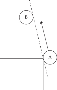
Figure 19.5
ORCA agent A is unable to continue turning around the corner without violating the sidedness constraint against B.
19.7 Gradient Methods Revisited
What we want from collision avoidance is for agents to find a consistent set of passing sides quickly, and ideally for that solution not to be too far from the optimum. When the situation changes—when a new agent arrives, or when existing agents change their minds about which way to go—we would like the system to adapt and find a new solution quickly, and for that new solution to look as much like the old one as possible. The key to that is weights.
19.7.1 Modifying Weights
In the original RVO paper, agents can be “weighted” with respect to each other—one agent can dodge by a larger or smaller percentage of the total required dodge than the other, as long as the two weights add up to 1 and the agents agree on what those weights are. But if we view RVO as a gradient method, as opposed to an instant, perfect collision solver, then it is clear that nothing forces that constraint. For instance, you could set both weights to 0.1, making agents slowly move out of each other’s way over many frames, but reliably settling into a stable configuration. Or you could set both weights to 0.9, causing agents to dodge sharply and exhibit the reciprocal oscillations that RVO was designed to avoid. (In fact, original-recipe VOs are simply a special case of RVO, with all weights set to 1.)
As mentioned, RVO is not quite a gradient method, because agents move after each iteration. In addition, if an upcoming collision has not yet been resolved, it just got a bit closer, and the problem just got a bit harder. If two agents are on a collision course, and the weights between them sum to anything less than 1.0, then their decisions each frame are guaranteed not to fully resolve the collision, and eventually they are guaranteed to veer off sharply and collide. If an algorithm can be said to “panic,” that’s what it looks like when an algorithm panics.
Low weights have their advantages, though. They tend to result in better solutions in the sidedness sense, particularly with large numbers of agents. But we need a way to cope with their tendency to fail asymptotically.
19.7.2 Substepping
Recall that as an algorithm for robot control, RVO relies on a cycle of steering, moving, and observing. One robot cannot react to another until that other robot has actually turned and started moving in another direction. But we have the benefit of knowing all agents’ velocities immediately after each steering step, even without moving the agents. We can use this knowledge to cheat, running multiple iterations of RVO between each movement step. The velocity outputs of one RVO substep become the velocity inputs of the next substep, and the positions remain unchanged.
This has a number of advantages. When groups of agents come upon each other, there is likely to be a number of frames of velocity flicker, as in the earlier example. Substepping allows that flicker to die down before velocities are presented to the animation system, giving the illusion that all agents made consistent choices the first time around.
Substepping also gives you more flexibility with your weights. Weightings that sum to less than 1.0 failed to resolve collisions, but they were good at finding the seeds of efficient solutions. During a step consisting of many substeps, you can start the weights low to smoothly hint toward an efficient solution, then ramp the weights up to 0.5 to fully settle into that solution along noncolliding trajectories.
If you’re familiar with stochastic optimization methods, you may find that sort of schedule, moving from the conservative to the abrupt, to be counterintuitive and backward. The goal here, though, is to converge reliably to a constraint-satisfying local optimum, rather than to converge reliably to the global optimum while maintaining constraints.
19.7.3 Time Horizons
ORCA’s cornering problem (getting stuck rather than changing passing side) is one example of a larger class of problems exhibited by VO methods when the assumption of constant preferred velocity is violated. Another, simpler form can be demonstrated with a single VO agent traveling north toward a goal point with a wall behind it. All northward velocities are blocked by the wall’s static velocity obstacle, so the agent can never reach the goal.
The original RVO reference library does not exhibit this problem, because it diverges from the paper and ignores collisions with static obstacles if they are further than the maximum stopping distance of the agent. Other RVO implementations address the problem by defining a maximum time-to-collision (TTC) beyond which projected collisions are ignored, causing the agent to slow as it approaches the obstacle, keeping its TTC above the threshold. The first approach assumes that the future policy is to come to a stop; the second approach assumes that the trajectory past the maximum TTC is too unpredictable to take into account. Both approaches are reasonable, but both are fairly arbitrary and can lead to collisions when agents end up squeezed between static obstacles and other agents.
In both cornering and approaching a goal in front of a wall, the basic issue is that agents are attempting to avoid a collision at a point that they would never reach. The cornering agent would veer off before getting to the collision point; the goal-approaching agent would stop first.
A more formal approach, then, would be to calculate the time at which the agent planned to stop at their goal, or to turn a corner, and to avoid collisions that would occur later than that time. The time horizon is specific to a given velocity candidate.
Time horizons are a little tricky to apply to cornering, because the agent does not plan to disappear after that but merely to turn a little bit. An agent currently rounding a corner has a time horizon approaching zero, yet should not ignore collisions entirely. Instead, one can construct a plane, perpendicular to the agent’s postcornering direction, which the agent never plans to cross. Collisions past that plane can safely be discarded, as shown in Figure 19.6.
This is not a perfect solution, as agents still fail to consider collisions that will occur after cornering. And it is not necessarily true that an agent will never cross their cornering plane: On occasion they may do so to avoid a collision right next to the corner. A better solution would involve predicting collisions along a space defined by the agent’s path, rather than world space. But because each agent has its own path, doing this in a way which would ensure proper reciprocation is, as far as we know, intractable in the general case.
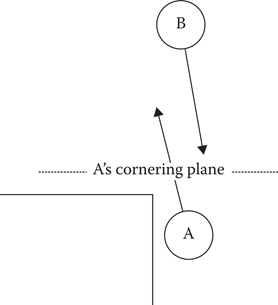
Figure 19.6
While A and B are on a colliding trajectory, the collision can be ignored as it would occur after A turns the corner.
Original VO methods treated the duty to avoid collisions as absolute. Making progress in their preferred directions was a secondary concern, only coming into play when choosing among a set of noncolliding and therefore valid trajectories. But as we have seen, avoiding far-off collisions is not always necessary or reasonable: Between the current step and the projected collision, a lot can happen, particularly when many agents are involved.
The RVO algorithm softens VO constraints, treating projected collisions as only one aspect when “scoring” a velocity candidate, making it a utility method. (ORCA does not soften its constraints in the same way: Its constraint relaxation is to produce at least one admissible velocity, not to allow colliding velocities when noncolliding velocities are available.) The base utility of a velocity candidate is calculated as the distance between the preferred velocity and the velocity candidate. Predicted collisions are treated as penalty terms reducing the utility of a velocity candidate, with the penalty term increasing as the collision becomes more imminent. If a velocity candidate is predicted to result in multiple collisions, the soonest collision can be used to determine the penalty, or each collision can generate a separate penalty term; the latter approach tends to push agents away from crowds decreasing congestion.
An additive formulation like this is motivated by practicality, not theory: It makes no guarantees of collision avoidance and increases the number of user-specified parameters, making tuning more difficult. Nevertheless, in practice, it is more effective than “absolute” VO methods at clearing congestion, as it discounts distant collisions, making it more reactive to closer ones.
19.8.1 Putting Sidedness Back In
The additive formulation does not automatically maintain sidedness (though substepping with low weights helps). However, nothing is stopping us from adding it as an additional penalty term. Simply calculate, for each velocity candidate, how many agents it changes the sidedness of; then add a penalty for each. Sidedness-change penalty terms should be scaled similarly to collision penalty terms; since they sometimes need to be applied to agents without projected collisions, though, the time to closest approach can be used instead of the TTC.
19.8.2 Progress and Energy Minimization
In the additive formulation above, the base utility of a velocity candidate is calculated as the distance from preferred velocity. This is not the only option: Another is rate of progress. In this formulation, the main metric is how fast an agent is making progress toward their goal, computed as the dot product of the velocity candidate with the unit-length preferred direction of travel. Compared to the distance metric, rate of progress encourages sideways dodging over slowing and tends to get agents to their goals sooner.
Rate of progress is an unrealistic utility from the point of view of actual human behavior. Consider that when moving from place to place, humans have the option of sprinting, yet generally move at a walking speed. Biomechanics researchers have explained this as a tendency toward energy minimization: A normal walking gait allows a human to reach their goal with the minimum expenditure of energy by maximizing the ratio of speed to power output. A rough approximation to the energy wasted by traveling at a nonpreferred velocity may be calculated as the squared distance between the preferred velocity (at preferred speed) and the velocity candidate; the squared term differentiates it from RVO’s approach. Agents using this utility calculation exhibit human-like trajectories, often slowing slightly to avoid a collision rather than turning left or right.
19.9 Putting It All Together: How to Develop a Practical Collision Avoidance System
Having a thorough knowledge of all the nuances and decisions and parameters involved in a VO-based collision avoidance system does not automatically give you the ability to make a perfect one. We are convinced that there is no perfect collision avoidance system, only one that works well with your scenarios, your needs, and your animation system. Developing such a system, like developing game systems in general, is an iterative process. There is a few important things you can do to increase the effectiveness of the process:
• Build up a library of collision avoidance scenarios, covering a variety of situations that your system will need to deal with. These should include all the factors you are likely to encounter in your game: static obstacles, cornering, multiple groups of agents, and so on. As you encounter problems with your system, make new scenarios that you can use to reproduce the problems, and test whether changes to your system have resolved them.
• Build up a library of collision avoidance algorithms too! As you make changes—either to the basic algorithms in use or the values you use for their parameters—keep the old algorithms around, not merely in source control but in active code. This will allow you to assess how well your iterative changes have improved collision avoidance quality, and it will allow you to test multiple approaches to resolving particular problems. Often later tweaks to a system will render earlier tweaks unnecessary, and keeping earlier versions around can help you recognize this and remove them, keeping your system as simple as possible.
• Put together a framework to automatically test each collision avoidance algorithm against each collision avoidance scenario. This isn’t quite as easy as it sounds: It is difficult to formulate criteria to determine whether a particular algorithm “passes” a particular test. As a first pass, you can simply check whether an algorithm succeeds in eventually bringing all agents to their goals without collisions along the way. You can compare two algorithms to determine which one gets agents to their goals sooner, but keep in mind that a difference of a few fractions of a second is not significant in a game scenario. It is important not to test collision avoidance in isolation: If your collision avoidance feeds into your animation system, rather than directly controlling agent positions, then you have to make your animation system part of the test rig in order to ensure accurate results. An automated testing rig is primarily useful for quickly checking for significant regressions in one or more test scenarios. It can also be used to quickly determine the optimal values for a set of control parameters.
• Don’t rely too heavily on your automated testing rig without doing frequent eyes-on testing of the results it is producing. Some collision avoidance algorithms can exhibit artifacts, which do not significantly impact the objective optimality of the results but which nevertheless look unrealistic to the player; velocity flicker is a prime example. You can try to come up with tests for this, but there’s no substitute for subjective evaluation.
Much of the popularity of VO methods can be traced to the ease of understanding them as prohibited shapes in velocity space. RVO in particular is seductively elegant in sharing the burden of collision avoidance between agents. But the success in practice of VO methods—particularly RVO—depends on subtler factors, and treating RVO as a purely geometric method makes it more difficult to leverage and maximize the effectiveness of these factors. So it is important to view VO methods through multiple lenses: As geometric solvers, as gradient methods, and as utility methods. There is nothing simple about this holistic approach, but collision avoidance is not a simple problem. Understanding both the nuances of the problem space and the complexity of the solution space is the key to developing a system that works for you.
van den Berg, J., Guy, S. J., Lin, M., and Manocha, D. 2011. Reciprocal n-body collision avoidance. In Robotics Research. Berlin, Germany: Springer, pp. 3–19.
van den Berg, J., Lin, M., and Manocha, D. 2008. Reciprocal velocity obstacles for real-time multi-agent navigation. Proceedings of the IEEE International Conference on Robotics and Automation (ICRA), 2008. http://gamma.cs.unc.edu/RVO/icra2008.pdf.