20

Optimization for Smooth Paths

Mark Langerak

20.1  Introduction

Path planning for games and robotics applications typically consists of finding the straight-line shortest path through the environment connecting the start and goal position. However, the straight-line shortest path usually contains abrupt, nonsmooth changes in direction at path apex points, which lead to unnatural agent movement in the path-­following phase. Conversely, a smooth path that is free of such sharp kinks greatly improves the realism of agent steering and animation, especially at the path start and goal positions, where the path can be made to align with the agent facing direction.

Generating a smooth path through an environment can be challenging because there are multiple competing constraints of total path length, path curvature, and static obstacle avoidance that must all be satisfied simultaneously. This chapter describes an approach that uses convex optimization to construct a smooth path that optimally balances all these competing constraints. The resulting algorithm is efficient, surprisingly simple, free of special cases, and easily parallelizable. In addition, the techniques used in this chapter serve as an introduction to convex optimization, which has many uses in fields as diverse as AI, computer vision, and image analysis. A source code implementation can be found on the book’s website (http://www.gameaipro.com).

20.2  Overview

The corridor map method introduced by Geraerts and Overmars, 2007 is used to construct an initial, nonoptimal path through the static obstacles in the environment. In the corridor map method, free space is represented by a graph where the vertices have associated disks. The centers of the disks coincide with the vertex 2D position, and the disk radius is equal to the maximum clearance around that vertex. The disks at neighboring graph vertices overlap, and the union of the disks then represents all of navigable space. See the leftside of Figure 20.1 for an example environment with some static obstacles in light gray and the corresponding corridor map graph.

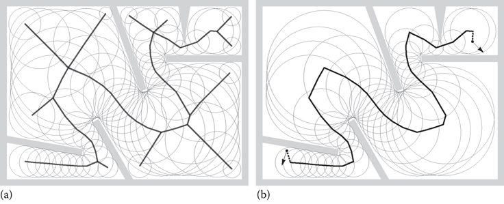
Figure 20.1
The corridor map (a) and a path between two points in the corridor map (b).

The corridor map method might be a lesser known representation than the familiar methods of a graph defined over a navigation mesh or over a grid. However, it has several useful properties that make it an excellent choice for the path smoothing algorithm described in this chapter. For one, its graph is compact and low density, so path-planning queries are efficient. Moreover, the corridor map representation makes it straightforward to constrain a path within the bounds of free space, which is crucial for the implementation of the path smoothing algorithm to ensure it does not result in a path that collides with static obstacles.

The rightside of Figure 20.1 shows the result of an A* query on the corridor map graph, which gives the minimal subgraph that connects the vertex whose center is nearest to the start position to the vertex whose center is nearest to the goal. The arrows in the figure denote the agent facing direction at the start position and the desired facing direction at the goal position. The subgraph is prepended and appended with the start and goal positions to construct the initial path connecting the start and the goal. Note that this initial path is highly nonoptimal for the purpose of agent path following since it has greatest clearance from the static obstacles, which implies that its total length is much longer than the shortest straight-line path.

Starting from this initial nonoptimal path state, the iterative algorithm described in this chapter evolves the path over multiple steps by successively moving the waypoints closer to an optimal configuration, that is, the path that satisfies all the competing constraints of smoothness, shortest total length, alignment with the start/goal direction and collision-free agent movement. The result is shown in the left of Figure 20.2.

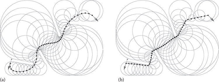
Figure 20.2
A smooth (a) and a straight-line path (b).

20.2.1  Definitions

In this section, we will define the mathematical notation used along with a few preliminary definitions. Vectors and scalars are denoted by lowercase letters. Where necessary, vectors use x, y superscripts to refer to the individual elements:

$a=\left(\begin{array}{c}{a}^x\\ a^y\end{array}\right)$

The vector dot product is denoted by angle brackets:

$\langle a,b\rangle =a^x{b}^x+a^y{b}^y$

The definition for the length of a vector uses double vertical bars:

${\Vert v\Vert }_2=\sqrt{\langle v,v\rangle }$

(The number 2 subscript on the double bars makes it explicit that the vector length is the L² norm of a vector.)

A vector space is a rather abstract mathematical construct. In the general sense, it consists of a set, that is, some collection of elements, along with corresponding operators acting on that set. For the path smoothing problem, we need two specific vector space definitions, one for scalar quantities and one for 2D vector quantities. These vector spaces are denoted by uppercase letters U and V, respectively:

$$\begin{gathered} U={\text{ℝ}}^n \\ V={\text{ℝ}}^{2n} \end{gathered}$$

The vector spaces U and V are arrays of length n, with vector space U an array of real (floating point) scalars, and V an array of 2D vectors. Individual elements of a vector space are referenced by an index subscript:

$a\in V:a_i$

In this particular example, a is an array of 2D vectors, and a_i is the 2D vector at index i in that array. Vector space operators like multiplication, addition, and so on, are defined in the obvious way as the corresponding pair-wise operator over the individual elements. The dot product of vector space V is defined as:

$a,b\in V:{\langle a,b\rangle }_V={\displaystyle {\sum }_{i=1}^n\langle a_i{b}_i\rangle }$

That is, the vector space dot product is the sum of the pair-wise dot products of the 2D vector elements. (The V subscript on the angle brackets distinguishes the vector space dot product from the vector dot product.)

For vector space V, we will make use of the norms:

$$\begin{gathered} v\in V:{\Vert v\Vert }_{V,1}={{\displaystyle {\sum }_{i=1}^n\Vert v_i\Vert }}_2 \\ v\in V:{\Vert v\Vert }_{V,2}=\sqrt{{\displaystyle {\sum }_{i=1}^n{\left({\Vert v_i\Vert }_2\right)}^2}} \\ v\in V:{\Vert v\Vert }_{V=\text{∞}}={\max }_{i=1}^n{\Vert v_i\Vert }_2 \end{gathered}$$

(The V subscript is added to make the distinction between vector and vector space norms clear.) Each of these three vector space norms are constructed similarly: they consist of an inner L² norm over the 2D vector elements, followed by an outer L¹, L², or $L^{\text{∞}}$ norm over the resulting scalars, respectively. In the case of the vector space L² norm, the outer norm is basically the usual definition of vector length, in this case a vector of length n. The vector space L¹ and $L^{\text{∞}}$ norms are generalizations of the familiar L² norm. The vector space L¹ norm is analogous to the Manhattan distance of a vector, and the $L^{\text{∞}}$ norm is the so-called max norm, which is simply the absolute max element.

An indicator function is a convenience function for testing set membership. It gives 0 if the element is in the set, otherwise it gives ∞ if the element is not in the set:

$I_s(x)=\{\begin{array}{cc}0& x\in S\\ \text{∞}& x\cancel{\in }S\end{array}$

The differencing operators give the vector offset between adjacent elements in V:

$$\begin{gathered} v\in V:{\text{δ}}^{+}{(v)}_i=\{\begin{array}{cc}(v_{i+1}-v_i)/h& i<n\\ 0& i=n\end{array} \\ v\in V:{\text{δ}}^{-}{(v)}_i=\{\begin{array}{cc}{v}_i/h& i=1\\ (v_i=v_{i-1})/h& 1<i<n\\ -v_{i=1}/h& i=n\end{array} \\ v\in V:{\text{δ}}^s(v)=-{\text{δ}}^{+}(v)+{\text{δ}}^{-}(v) \end{gathered}$$

The forward differencing operator ${\text{δ}}^{+}$ gives the offset from the 2D vector at index i to the next vector at index i+1. The boundary condition at index i = n is needed because then there is no “next” vector, and there the offset is set to 0. Similarly, the backward differencing operator ${\text{δ}}^{-}$ gives the offset from the vector at index i to the previous vector at index i–1, with boundary conditions at i=1, and i=n to ensure that ${\text{δ}}^{+}$ and ${\text{δ}}^{-}$ are adjoint. The sum-differencing operator ${\text{δ}}^s$ is the vector addition of the vector offsets ${\text{δ}}^{+}$ and ${\text{δ}}^{-}$. The scalar h is a normalization constant to enforce scale invariance. It depends on the scale of the 2D coordinate space used, and its value should be set to the average distance between neighboring graph vertices.

20.3  Path Smoothing Energy Function

An optimization problem consists of two parts: an energy (aka cost) function and an optimization algorithm for minimizing that energy function. In this section, we will define the energy function; in the following sections, we will derive the optimization algorithm.

The path smoothing energy function gives a score to a particular configuration of the path waypoints. This score is a positive number, where large values mean the path is “bad,” and small values mean the path is “good.” The goal then is to find the path configuration for which the energy function is minimal. The choice of energy function is crucial. Since it effectively will be evaluated many times in the execution of the optimization algorithm, it needs to be simple and fast, while still accurately assigning high energy to nonsmooth paths and low energy to smooth paths.

As described in the introduction section, the fundamental goal of the path smoothing problem is to find the optimal balance between path smoothness and total path length under the constraint that the resulting path must be collision free. Intuitively, expressing this goal as an energy function leads to a sum of three terms: a term that penalizes (i.e., assigns high energy) to waypoints where the path has sharp kinks, a term that penalizes greater total path length, and a term that enforces the collision-free constraint. In addition, the energy function should include a scaling factor to enable a user-controlled tradeoff between overall path smoothness and total path length. The energy function for the path smoothing problem is then as follows:

$$\begin{gathered} w\in U,v\in V:E\text{(}v)=\frac{1}{2}{\left({\Vert w{\text{δ}}^s(v)\Vert }_{v,2}\right)}^2+{\Vert {\text{δ}}^{+}(v)\Vert }_{v,2}+I_C(v) \\ C=\left\{v,c\in V,r\in U:{\Vert (v-c)/r\Vert }_{v,\text{∞}}\le 1\right\} \end{gathered}$$

(20.1)

Here, v are the path waypoint positions, and w are per waypoint weights. Set C represents the maximal clearance disk at each waypoint, where r are the disk centers, and c are the radii. (Note that this path smoothing energy function is convex, so there are no local minima that can trap the optimization in a nonoptimal state, and the algorithm is therefore guaranteed to converge on a globally minimal energy.)

The first term in the energy function gives a high score to nonsmooth paths by penalizing waypoints where the path locally deviates from a straight line. See Figure 20.3 for a visual representation, where the offsets ${\text{δ}}^s$, ${\text{δ}}^{+}$, and ${\text{δ}}^{-}$ for waypoint 3 are drawn with arrows. The dark arrow shows offset vector ${\text{δ}}^s$, and it can be seen from the left and the right Figure 20.3 that its length is relative to how much waypoint v₃ deviates from the straight line connecting v₂ and v₄. The offset vector ${\text{δ}}^s$ length is squared to penalize sharp kinks progressively more than shallow ones, which forces the optimization algorithm to spread out sharp kinks over adjacent waypoints, leading to an overall smoother path.

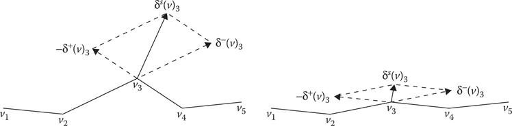
Figure 20.3
A visual representation of the model.

The second term in the energy function gives a higher score to greater total path length by summing the lengths of the ${\text{δ}}^{+}$ vectors. It effectively forces path waypoints to be closer together, resulting in a path that has a shorter total length and which is thus more similar to the straight-line shortest path connecting the start and goal.

Set C acts as a constraint on the optimization problem to ensure the path is collision free. Due to the max norm in the definition, the indicator function I_C gives infinity when one or more waypoints are outside their corresponding maximal clearance disk, otherwise it gives zero. A path that has waypoints that are outside their corresponding maximal clearance disk will have infinite energy therefore, and thus can obviously never be the minimal energy state path.

The required agent facing directions at the start and goal positions are handled by extending the path at both ends with a dummy additional waypoint, which are shown by the small circles in Figure 20.2. The position of the additional waypoints is determined by subtracting or adding the facing direction vector to the start and goal positions. These dummy additional waypoints as well as the path start and goal position are assigned a zero radius clearance disk. This constrains the start/goal positions from shifting around during optimization and similarly prevents the start/goal-facing direction from changing during optimization.

The per waypoint weights w allow a user-controlled tradeoff between path smoothness and overall path length, where lower weights favor short paths and higher weights favor smooth paths. In the limit, when all the weights are set to zero, the energy function only penalizes total path length, and then the path optimization will result in the shortest straight-line path as shown in the right of Figure 20.2. In practice, the weights near the start and goal are boosted to improve alignment of the path with the required agent facing direction. This is done using a bathtub-shaped power curve:

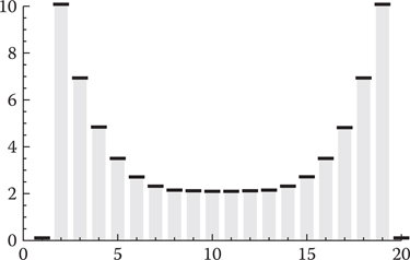
Figure 20.4
A waypoint weight curve.

$w=\{\begin{array}{cc}{w}_m+(w_s-w_m){\left(\frac{-2(i-2)}{n-3}+1\right)}^4& 2\le i\le \frac{n}{2}\\ w_m+(w_e-w_m){\left(\frac{-2(i-2)}{n-3}+1\right)}^4& \frac{n}{2}<i\le -1\\ 0& otherwise\end{array}$

The scalars w_s and w_e are the values of the weight for the start and goal position waypoints, respectively. The end position weights taper off with a power curve to weight w_m at the middle of the path. Index i=1 and i=n are the dummy waypoints for the agent facing direction, and there the weights are zero. Figure 20.4 shows a plot for an example weight curve with w_s=w_e=10, w_m=2, and n=20.

20.4  Optimization Algorithm

Minimizing the energy function (Equation 20.1) is a challenging optimization problem due to the discontinuous derivative of the vector space norms and the hard constraints imposed by the maximal clearance disks. In this context, the path smoothing problem is similar to optimization problems found in many computer vision applications, which likewise consist of discontinuous derivatives and have hard constraints. Recent advances in the field have resulted in simple and efficient algorithms that can effectively tackle such optimization tasks; in particular, the Chambolle–Pock preconditioned primal-dual algorithm described in Chambolle and Pock 2011, and Pock and Chambolle 2011 has proven very effective in computer vision applications due to its simple formulation and fast convergence. Furthermore, it generalizes and extends several prior known optimization algorithms such as preconditioned ADMM and Douglas–Rachford splitting, leading to a very general and flexible algorithm.

The algorithm requires that the optimization problem has a specific form, given by:

$\underset{v\in V}{\min }\left\{E_p(v)=F(K\cdot v)+G(v)\right\}$

(20.2)

That is, it minimizes some variable v for some energy function E_p, which itself consists of a sum of two (convex) functions F and G. The parameter to function F is the product of a matrix K and variable v. The purpose of matrix K is to encode all the operations on v that depend on adjacent elements. This results in a F and G function that are simple, which is necessary to make the implementation of the algorithm feasible. In addition, matrix K is used to compute a bound on the step sizes, which ensures the algorithm is stable.

The optimization problem defined by Equation 20.2 is rather abstract and completely generic. To make the algorithm concrete, the path smoothing energy function (Equation 20.1) is adapted to the form of Equation 20.2 in multiple steps. First, we define the functions F₁, F₂, and G to represent the three terms in the path smoothing energy function:

$F_1(v)=\frac{1}{2}{\left({\Vert v\Vert }_{V,2}\right)}^2,F_2(v)={\Vert v\Vert }_{V,2},G(v)=I_C(v)$

In the path smoothing energy function (Equation 20.1), the operators $w{\text{δ}}^s$ and ${\text{δ}}^{+}$ act on adjacent elements in v, so these are the operators that must be encoded as matrix K. As an intermediate step, we first define the two submatrices $K_1=w{\text{δ}}^{s}and{K}_{\text{2}}={\text{δ}}^{+}$. We can then state the equivalence:

$K_1\cdot v=w{\text{δ}}^s(v),K_2\cdot v={\text{δ}}^{+}(v)$

Substituting these as the parameters to functions F₁ and F₂ results in:

$F_1(K_1\cdot v)=\frac{1}{2}{\left({\Vert w{\text{δ}}^s(v)\Vert }_{V,2}\right)}^2,F_2(K_2\cdot v)={\Vert {\text{δ}}^{+}(v)\Vert }_{V,2}$

which leads to the minimization problem:

$\underset{v\in V}{\min }\left\{E_p(v)=F_1(K_1\cdot v)+F_2(K_2\cdot v)+G(v)\right\}$

This is already largely similar to the form of Equation 20.2, but instead of one matrix K and one function F, we have two matrices K₁ and K₂, and two functions F₁ and F₂. By “stacking” these matrices and functions, we can combine them into a single definition to make the path smoothing problem compatible with Equation 20.2:

$K=\left(\begin{array}{c}{K}_1\\ K_2\end{array}\right),F(K\cdot v)=\left(\begin{array}{c}{F}_1(K_1\cdot v)\\ F_2(K_2\cdot v)\end{array}\right)$

Next, matrix K is defined to complete the derivation of the path smoothing problem. For the matrix-vector product $K\cdot v$, it is necessary to first “flatten” v into a column vector ${(v_1^x,v_1^y,v_1^x{v}_2^y,\cdot \cdot \cdot ,v_n^x{v}_n^y)}^T$. Then K is a $4n\times 2n$-dimensional matrix where rows 1 to 2n encode the $w{\text{δ}}^s$ operator, and rows 2n+1 to 4n encode δ⁺. See Figure 20.5 for an example with n = 4. From Figure 20.5, it is easy to see that applying K ⋅ v is the same operation as wδ^s(v) and δ⁺(v).

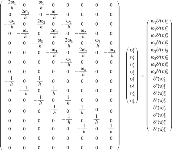
Figure 20.5
Matrix K for n = 4.

Note that in practice, the definition of matrix K is only needed to analyze the optimization algorithm mathematically; it is not used in the final implementation. The matrix is very large and sparse, so it is obviously much more efficient to simply use the operators wδ^s and δ⁺ in the implementation instead of the actual matrix-vector product K ⋅ v.

Instead of solving the minimization problem (Equation 20.2) directly, the Chambolle–Pock algorithm solves the related min–max problem:

$\underset{v\in V}{\text{min}}\underset{p\in V}{\text{max}}\left\{E_{pd}\left(v\right)={\langle K\cdot v,p\rangle }_V+G\left(v\right)-F^{*}\left(p\right)\right\}$

(20.3)

The optimization problems Equations 20.2 and 20.3 are equivalent: minimizing Equation 20.2 or solving the min–max problem (Equation 20.3) will result in the same v. The original optimization problem (Equation 20.2) is called the “primal,” and Equation 20.3 is called the “primal-dual” problem. Similarly, v is referred to as the primal variable, and the additional variable p is called the dual variable.

The concept of duality and the meaning of the star superscript on F* are explained further in the next section, but at first glance it may seem that Equation 20.3 is a more complicated problem to solve than Equation 20.2, as there is an additional variable p, and we are now dealing with a coupled min–max problem instead of a pure minimization. However, the additional variable enables the algorithm, on each iteration, to handle p separately while holding v constant and to handle v separately while holding p constant. This results in two smaller subproblems, so the system as a whole is simpler.

In the case of the path smoothing problem, we have two functions F₁ and F₂, so we need one more dual variable q, resulting in the min–max problem:

$\underset{v\in V}{\text{min}}\underset{p,q\in V}{\text{max}}\left\{E_{pd}\left(v\right)={\langle K\cdot v,\left(\begin{array}{c}p\\ q\end{array}\right)\rangle }_V+G\left(v\right)-F_1^{\ast }\left(p\right)-F_2^{\ast }\left(q\right)\right\}$

Note that, similar to what was done to combine matrices K₁ and K₂, the variables p and q are stacked to combine them into a single definition (p,q)^T.

20.4.1  Legendre–Fenchel Transform

The Legendre–Fenchel (LF) transform takes a function f and puts in a different form. The transformed function is denoted with a star superscript, f*, and is referred to as the dual of the original function f. Using the dual of a function can make certain kinds of analysis or operations much more efficient. For example, the well-known Fourier transform takes a time domain signal and transforms (dualizes) it into a frequency domain signal, where convolution and frequency analysis are much more efficient. In the case of the LF transform, the dualization takes the form of a maximization:

$f^{\ast }\left(k\right)=\underset{x\in {\text{ℝ}}^n}{\text{max}}\left\{\langle k,x\rangle -f\left(x\right)\right\}$

(20.4)

The LF transform has an interesting geometric interpretation, which is unfortunately out of scope for this chapter. For more information, see Touchette 2005, which gives an excellent explanation of the LF transform. Here we will restrict ourselves to simply deriving the LF transform for the functions F₁ and F₂ by means of the definition given by Equation 20.4.

20.4.1.1  Legendre–Fenchel Transform of F₁

Substituting the definition of F₁ for f in Equation 20.4 results in:

$p\in V:F_1^{\ast }\left(p\right)=\underset{x\in V}{\max }\left\{{\langle p,x\rangle }_V-\frac{1}{2}{\langle x,x\rangle }_V\right\}$

(20.5)

The maximum occurs where the derivative w.r.t. x is 0:

$\frac{\partial }{\partial x}\left({\langle p,x\rangle }_V-\frac{1}{2}{\langle x,x\rangle }_V\right)=0\Rightarrow p-x=0$

So the maximum of F₁ is found where x = p. Substituting this back into Equation 20.5 gives:

$F_1^{\ast }\left(p\right)=\frac{1}{2}{\langle p,p\rangle }_V$

20.4.1.2  Legendre–Fenchel Transform of F₂

Substituting the definition of F₂ for f in Equation 20.4 gives:

$q\in V:F_2^{\ast }\left(q\right)=\underset{x\in V}{\max }\left\{{\langle q,x\rangle }_V-{\Vert x\Vert }_{V,2}\right\}$

(20.6)

The ${\langle q,x\rangle }_V$ term can be (loosely) seen as the geometric dot product of q and x. This is maximized when q and x are “geometrically coincident,” that is, they are a scalar multiple of each other. When q and x are coincident, then by the definition of the dot product ${\langle q,x\rangle }_V={\Vert q\Vert }_{V,2}{\Vert x\Vert }_{V,2}$ holds. Substituting this back into Equation 20.6 gives:

$F_2^{\ast }\left(q\right)=\underset{x\in V}{\max }\left\{{\Vert q\Vert }_{V,2}{\Vert x\Vert }_{V,2}-{\Vert x\Vert }_{V,2}\right\}$

This makes it obvious that when ${\Vert q\Vert }_{V,2}\le 1$, the maximum that can be attained for Equation 20.6 is 0; otherwise when ${\Vert q\Vert }_{V,2}>1$, the maximum goes to ∞. This is conveniently expressed as the indicator function of an additional set Q:

$\begin{array}{cc}{F}_2^{\ast }\left(q\right)=I_Q\left(q\right),& Q=\left\{q\in V:{\Vert q\Vert }_{V,2}\le 1\right\}\end{array}$

20.4.2  Proximity Operator

In the previous section, we derived the dual functions $F_1^{\ast }$ and $F_2^{\ast }$. Before we can define the path smoothing algorithm, we also need to derive the so-called proximity operator for functions $F_1^{\ast }$, $F_2^{\ast }$, and G. The proximity operator bounds a function from below with a quadratic in order to smooth out discontinuities in the derivative. This ensures the optimization converges on the minimum without getting trapped in an oscillation around the minimum. See Figure 20.6 for a simple example where the solid line is the original function with a discontinuous derivative, and the dotted lines are quadratic relaxations of that function. The general definition of the proximity operator is given by the minimization:

$pro{x}_{f,\text{τ}}\left(x\right)=\underset{y\in {\text{ℝ}}^n}{\text{argmin}}\left\{f\left(y\right)+\frac{1}{2\text{τ}}{\left({\Vert y-x\Vert }_2\right)}^2\right\}$

(20.7)

where the parameter τ controls the amount of relaxation due to the quadratic.

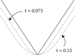
Figure 20.6
Quadratic relaxation.

20.4.2.1  Proximity Operator of $F_1^{\ast }$

Substituting $F_1^{\ast }$ into Equation 20.7 gives:

$p\in V:pro{x}_{F_1^{\ast },\text{σ}}{\left(p\right)}_i=\underset{y\in {\text{ℝ}}^2}{\text{argmin}}\left\{\frac{\langle y,y\rangle }{2}+\frac{1}{2\text{σ}}{\left({\Vert y-p_i\Vert }_2\right)}^2\right\}$

Note that the proximity operator $F_1^{\ast }$ is point-wise separable, meaning that it can be defined in terms of the individual elements p_i. The point-wise separation is possible due to the fact that the operations that depend on adjacent elements of v are encoded in matrix K, and as a consequence, there similarly is no mutual dependence between adjacent elements of p here. This simplifies the derivation of the proximity operator greatly. (In fact, without point-wise separation, the derivation of the proximity operator would not be feasible.) The minimum occurs where the derivative w.r.t. y is 0:

$\frac{\partial }{\partial y}\left(\frac{\langle y,y\rangle }{2}-\frac{1}{2\text{σ}}\langle y-p_i,y-p_i\rangle \right)=0\Rightarrow y+\frac{y-p_i}{\text{σ}}=0$

Solving this equation for y results in:

$p\in V:pro{x}_{F_1^{\ast },\text{σ}}{\left(p\right)}_i=\frac{p_i}{1+\text{σ}}$

20.4.2.2  Proximity Operator of $F_2^{\ast }$

Substituting $F_2^{\ast }$ into Equation 20.7 gives:

$q\in V:pro{x}_{F_{2\text{}}^{\ast }\text{},\text{μ}}\left(q\right)=\underset{y\in V}{\text{argmin}}\left\{I_Q\left(y\right)+\frac{1}{2\text{μ}}{\left({\Vert y-q\Vert }_{V,2}\right)}^2\right\}$

The indicator function I_Q completely dominates the minimization—it is 0 when $y\in Q$, otherwise it is in which case the minimum does not exist. So to attain a minimum, y must be member of Q. Hence, the solution to the proximity operator for $F_2^{\ast }$ consists of finding the nearest y to q that is also a member of Q (in convex optimization terms, this is called “projecting” y onto Q.) If y is in Q, this is simply y itself; otherwise y is divided by its L² norm, so it satisfies ${\Vert q\Vert }_{V,2}\le 1$. Thus:

$q\in V:pro{x}_{F_2^{\ast },\text{μ}}\left(q\right)=\frac{q}{\text{max}\left(1,{\Vert q\Vert }_{V,2}\right)}$

20.4.2.3  Proximity Operator of G

Substituting G into Equation 20.7 gives:

$v\in V:pro{x}_{G,\text{τ}}\left(v\right)=\underset{y\in V}{\arg \min }\left\{I_C\left(y\right)+\frac{1}{2\text{τ}}{\left({\Vert y-v\Vert }_{V,2}\right)}^2\right\}$

Similar to the proximity operator of $F_2^{\ast }$ above, here the indicator function L_C dominates the minimization, and so the solution consists of finding the nearest y that is in C. The problem is point-wise separable, and the solution is given as the point inside the maximal clearance disk with center c_i and radius r_i that is nearest to v_i:

$v\in V:pro{x}_{G,\text{τ}}{\left(v\right)}_i=c_i+\left(v_i-c_i\right)\frac{r_i}{\max \left(r_i,{\Vert v_i-c_i\Vert }_2\right)}$

20.4.3  The Chambolle–Pock Primal-Dual Algorithm for Path Smoothing

The general preconditioned Chambolle–Pock algorithm consists of the following steps:

$\begin{array}{c}{p}^{k+1}=pro{x}_{F^{\ast },\text{Σ}}\left(p^k+\text{Σ}\cdot K\cdot {\widehat{v}}^k\right)\\ v^{k+1}=pro{x}_{G,\text{Τ}}\left(v^k-\text{Τ}\cdot K^T\cdot p^{k+1}\right)\\ {\widehat{v}}^{k+1}=2v^{k+1}-v^k\end{array}$

(20.8)

These are the calculations for a single iteration of the algorithm, where the superscripts k and k+1 refer to the value of the corresponding variable at the current iteration k and the next iteration k+1. The implementation of the algorithm repeats the steps (Equation 20.8) multiple times, with successive iterations bringing the values of the variables closer to the optimal solution. In practice, the algorithm runs for some predetermined, fixed number of iterations that brings the state of variable v sufficiently close to the optimal value. Prior to the first iteration k=0, the variables are initialized as $p^0=q^0=0$ and $v^0={\widehat{v}}^0=c$. The diagonal matrices Σ and T are the step sizes for the algorithm, which are defined below.

The general algorithm (Equation 20.8) is adapted to the path smoothing problem by substituting the definitions given in the previous sections: the differencing operators $w{\text{δ}}^s$ and δ⁺ are substituted for K,p, is substituted with the stacked variable (p,q)^T, and $pro{x}_{F^{\ast },\text{Σ}}$ is substituted with $pro{x}_{F_1^{\ast },\text{σ}}$ and $pro{x}_{F_2^{\ast },\text{μ}}$. Then the final remaining use of matrix K is eliminated by expanding the product:

$K^T\cdot {\left(\begin{array}{c}p\\ q\end{array}\right)}^{k+1}\Rightarrow w{\text{δ}}^s\left(p^{k+1}\right)-{\text{δ}}^{-}\left(q^{k+1}\right)$

This results in the path smoothing algorithm:

$\begin{array}{c}{p}^{k+1}=pro{x}_{F_1^{\ast },\text{σ}}\left(p^k+\text{σ}w{\text{δ}}^s\left({\widehat{v}}^k\right)\right)\\ q^{k+1}=pro{x}_{F_2^{\ast },\text{μ}}\left(q^k+\text{μ}{\text{δ}}^{+}\left({\widehat{v}}^k\right)\right)\\ v^{k+1}=pro{x}_{G,\text{τ}}\left(v^k-\text{τ}\left(w{\text{δ}}^s\left(p^{k+1}\right)-{\text{δ}}^{-}\left(q^{k+1}\right)\right)\right)\\ {\widehat{v}}^{k+1}=2v^{k+1}-v^k\end{array}$

By substituting K and K^T with their corresponding differencing operators, the step size matrices Σ and T are no longer applicable. Instead, the step sizes are now represented by the vectors $\text{σ},\text{μ},\text{τ}\in U$, which are the diagonal elements of matrices Σ and T. As proven in Pock and Chambolle 2011, deriving the step-size parameters $\text{σ},\text{μ},\text{τ}$ as sums of the rows and columns of matrix K leads to a convergent algorithm:

$\begin{array}{ccc}{\text{σ}}_i=\frac{1}{\text{β}{{{\displaystyle \sum }}^{\text{}}}_{j=1}^{2n}{K}_1{{\text{}}_{{\text{}}_{i,j}}}^{\text{α}}},& {\text{μ}}_i=\frac{1}{\text{β}{{{\displaystyle \sum }}^{\text{}}}_{j=1}^{2n}{K}_2{{\text{}}_{{\text{}}_{i,j}}}^{\text{α}}},& {\text{τ}}_i=\frac{\text{β}}{{{{\displaystyle \sum }}^{\text{}}}_{j=1}^{4n}{K}_{j,i}{\text{}}^{2-\text{α}}}\end{array}$

Expanding the summation gives:

${\text{σ}}_i=\frac{h^{\text{α}}}{\left(2+2^{\text{α}}\right)\text{β}{w}_i{\text{}}^{\text{α}}},{\text{μ}}_i=\frac{h^{\text{α}}}{2\text{β}},{\text{τ}}_i=\frac{\text{β}{h}^{2-\text{α}}}{2+w_{i-1}{\text{}}^{2-\text{α}}+{\left(2w_i\right)}^{2-\text{α}}+w_{i+1}{\text{}}^{2-\text{α}}}$

(20.9)

(Note that μ_i is a constant for all i.) The scalar constants 0 < α < and β > 0 balance the step sizes to either larger values for σ,μ or larger values for τ. This causes the algorithm to make correspondingly larger steps in either variable p,q or variable v on each iteration, which affects the overall rate of convergence of the algorithm. Well-chosen values for α,β are critical to ensure an optimal rate of convergence. Unfortunately, optimal values for these constants depend on the particular waypoint weights used and the average waypoint separation distance h, so no general best value can be given, and they need to be found by experimentation. Note that the Equations 20.9 are valid only for 2 < i < n – 1, that is, they omit the special cases for the step size at i = 1 and i = n. They are omitted because in practice, the algorithm only needs to calculate elements 2 < i < n – 1 for p, q, v and $\widehat{v}$ on each iteration. This is a consequence of extending the path at either end with two dummy additional waypoints for the agent facing direction. Since these additional waypoints are assigned a zero radius clearance disk, their position remains fixed on each iteration. Their contribution to the path energy is therefore constant and does not need to be calculated. Restricting the algorithm implementation to elements 2 < i < n – 1 eliminates all special cases for the boundary conditions of operator δ^s, δ⁺, δ^–, and the step sizes.

The leftside of Figure 20.7 shows the state of the path as it evolves over 100 iterations of the algorithm. Empirically, the state rapidly converges to a smooth path after only a few initial iterations. Subsequent iterations then pull the waypoints closer together and impose a uniform distribution of waypoints over the length of the path. The rightside of Figure 20.7 is a plot of the value of the energy function (Equation 20.1) at each iteration, which shows that the energy decreases (however not necessarily monotonically) on successive iterations.

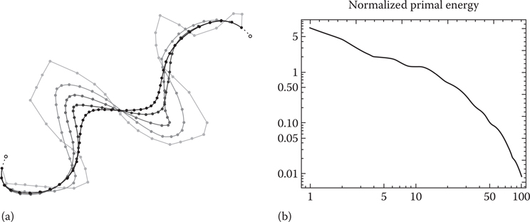
Figure 20.7
(a) Path evolution and (b) energy plot.

20.5  Conclusion

In this chapter, we have given a detailed description of an algorithm for path smoothing using iterative minimization. As can be seen from the source code provided with this chapter on the book’s website (http://www.gameaipro.com), the implementation only requires a few lines of C++ code. The computation at each iteration consists of simple linear operations, making the method very efficient overall. Moreover, since information exchange for neighboring waypoints only occurs after each iteration, the algorithm inner loops that update the primal and dual variables are essentially entirely data parallel, which makes the algorithm ideally suited to a GPGPU implementation.

Finally, note that this chapter describes just one particular application of the Chambolle–Pock algorithm. However, the algorithm itself is very general and can be adapted to solve a wide variety of optimization problems. The main hurdle in adapting it to new applications is deriving a suitable model, along with its associated Legendre–Fenchel transform(s) and proximity operators. Depending on the problem, this may be more or less challenging. However, once a suitable model is found, the resulting code is invariably simple and efficient.

References

Chambolle, A. and T. Pock. 2011. A first-order primal-dual algorithm for convex problems with applications to imaging. Journal of Mathematical Imaging and Vision, 40(1), 120–145.

Geraerts, R. and M. Overmars. 2007. The corridor map method: A general framework for real-time high-quality path planning. Computer Animation and Virtual Worlds, 18, 107–119.

Pock, T. and A. Chambolle. 2011. Diagonal preconditioning for first order primal-dual algorithms in convex optimization. IEEE International Conference on Computer Vision (ICCV), Washington, DC, pp. 1762–1769.

Touchette, H. 2005. Legendre-Fenchel transforms in a nutshell. School of Mathematical Sciences, Queen Mary, University of London. http://www.physics.sun.ac.za/~htouchette/archive/notes/lfth2.pdf (accessed May 26, 2016).