
Goal bounding is a pathfinding optimization technique that can speed up A* by roughly eight times on a grid (Rabin and Sturtevant 2016), however, it is applicable to any graph search space, including waypoint graphs or navmeshes (navigation meshes). Goal bounding is not a search algorithm itself, but rather a method to prune the search space, thus radically reducing the number of nodes that need to be considered to find the goal. This is accomplished by preprocessing the search space offline and using the precomputed data to avoid exploring many nodes that do not lead to the goal.
This chapter will introduce the goal-bounding concept, walk through the runtime code, and then show the necessary preprocessing steps. We will then discuss experimental data that shows the effective speed-up to a standard A* implementation.
22.1.1 Goal-Bounding Constraints
Goal bounding has three constraints that limit whether it is appropriate to use in your game:
1. Map constraint: The map must be static and cannot change during gameplay. Nodes and edges cannot be added or deleted.
2. Memory constraint: For each node in the map, there is a requirement of four values per node edge in memory during runtime. Grid nodes have eight edges, and navmesh nodes have three edges. Typically, each value is 2 bytes.
3. Precomputation constraint: The precomputation is O(n2) in the number of nodes. This is a costly computation and can take from 5 minutes to several hours per map. This is performed offline before the game ships.
The most important constraint is that your game maps must be static. That is to say that the nodes and edges in your search space must not change during gameplay, and the cost to go from one node to another must also not change. The reason is that connection data must be precomputed. Changing a single node, edge, or cost would invalidate all of the precomputed data. Because the precomputed data takes so long to create, it is not feasible to dynamically rerun the computation if the map changes.
The other primary constraint is that goal bounding requires extra memory at runtime for the precomputed data. For every node, there has to be four values per edge leading to another node. On a grid, each node has eight edges (or connections) to other nodes, so the necessary data for a grid search space are 32 values per node. On a navmesh, typically each poly node has three edges, so the necessary data for a navmesh search space are 12 values per poly node. Typically, these values will need to be 2 bytes each, but for smaller maps, 1 byte each might suffice (e.g., a grid map with a height and width less than 256).
Lastly, a minor constraint is that each map must be precomputed offline, which takes time. The precomputation algorithm is O(n2) in the number of total nodes on the map. For example, a very large 1000 × 1000 grid map would have 1 million nodes, requiring 1,000,0002 or 1 trillion operations during precomputation for that map. Depending on the map size, this can take between 5 minutes and several hours per map. It is computationally demanding enough that you could not precompute the data at runtime. However, there are optimizations to Dijkstra for uniform cost grids, such as Canonical Dijkstra that can make this computation much faster (Sturtevant and Rabin 2017).
Fortunately, there are many things that are not constraints for goal bounding. For example, the following aspects are very flexible:
1. Goal-bounding works on any graph search space, including grids, waypoint graphs, quadtrees, octrees, and navmeshes, as long as the points in these graphs are associated with coordinates in space.
2. Goal bounding can be applied to any search algorithm (A*, Dijkstra, JPS+, etc.). Typically, A* is best for games, but goal bounding can work with Dijkstra and works extremely well with JPS+ (a variant of A* only for uniform cost grids).
3. The map can have nonuniform costs between nodes, meaning the cost to go from one node to another node can vary as long as it does not change during the game. Some algorithms like JPS+ have restrictions such that they only work on uniform cost grids, where the cost between grid squares must be consistent.
The name goal bounding comes from the core concept. For each edge adjacent to a node, we precompute a bounding box (4 values) that contains all goals that can be optimally reached by exploring this edge. At runtime, we only explore this node’s edge if the goal of the search lies in the bounding box. Reread those last two sentences again, because this is the entire runtime algorithm.
In Figure 22.1, consider the node marked with a circle. The gray nodes in the left map can all be reached optimally by exploring the left edge of the circle node (we will discuss later how this is computed). The gray bounding box in the right map contains all of the gray nodes from the left map and represents what needs to be precomputed (4 values that define a bounding box: left, right, top, and bottom). This precomputed bounding box is stored in the left edge of the circle node. At runtime, if we are at the circle node and considering exploring the left edge, we would check to see if the goal lies in the bounding box. If it does, we explore this edge as is normally done in the A* algorithm. If the goal does not lie in the bounding box, we skip this edge (the edge is pruned from the search).
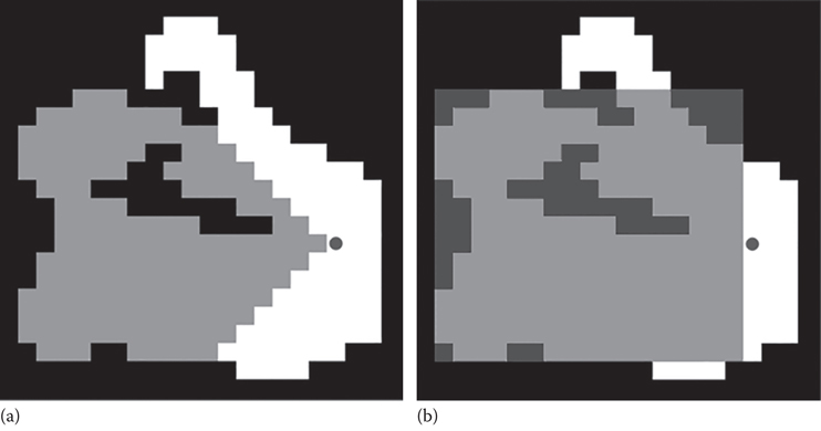
Figure 22.1
The map in (a) shows all of the nodes (in gray) that can be reached optimally by exploring the left edge of the circle node. The map in (b) shows a bounding box of the nodes in the left image. This bounding box is stored in the left edge of the circle node.
Goal bounding can be similarly applied to navmeshes. Consider the black node in the navmesh in Figure 22.2. The dark gray nodes can be reached optimally through the bottom right edge of the black node. Figure 22.3 shows a bounding box around these nodes. This is the identical concept as shown on the grid in Figure 22.1.
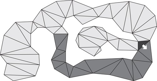
Figure 22.2
Nodes marked in dark gray can be reached optimally from exploring the bottom right edge of the black node. All other nodes in the map can only be reached optimally by exploring either the top edge or the left edge of the black node.
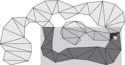
Figure 22.3
The bounding box containing all nodes that can be reached optimally from the bottom right edge of the black node. In goal bounding, this bounding box is stored in the bottom right edge of the black node.
For A* with goal bounding to work, it is assumed that every node edge has a precomputed bounding box containing all nodes that can be reached optimally through that edge. With this data, the only addition to the runtime is a simple check, as shown in bold in Listing 22.1.
Listing 22.1. A* algorithm with the goal bounding check added (in bold).
procedure AStarSearch(start, goal)
{
Push (start, openlist)
while (openlist is not empty)
{
n = PopLowestCost (openlist)
if (n is goal)
return success
foreach (neighbor d in n)
{
if (WithinBoundingBox(n, d, goal))
{
// Process d in the standard A* manner
}
}
Push (n, closedlist)
}
return failure
}
The goal-bounding check in Listing 22.1 tests whether we really want to explore a neighboring node, through the parent node’s edge. If the check succeeds (the goal of the search is within the bounding box), then the search algorithm proceeds as normal through this edge. If the check fails, the edge is pruned by simply skipping it. This has the dramatic effect of not exploring that edge and all of the subsequent edges, thus pruning huge swaths of the search space. This accounts for goal bounding’s dramatic speed improvement (Rabin and Sturtevant 2016). Note that this goal-bounding check can be inserted into any search algorithm at the point the algorithm is considering a neighboring node.
Precomputation consists of computing a bounding box for every edge of every node. If we can design an algorithm that computes this information for a single node, then it is just a matter of iterating that algorithm over every node in the map. In fact, the problem is embarrassingly parallel in which we can kick off one thread per node in the map, since each node’s bounding boxes are independent of all other node’s bounding boxes. With enough cores running the threads, the precomputation time can be greatly minimized.
To compute the bounding boxes for all edges of a single node, we need to use a slightly enhanced Dijkstra search algorithm. Recall that Dijkstra is the same as A*, but the heuristic cost is zero. This causes the search to spread out evenly, in cost, away from the starting point. For our purposes, we will start the Dijkstra search at our single node and give it no destination, causing it to search all nodes in the map, as if it was performing a floodfill.
Using Dijkstra to floodfill, the map has the effect of marking every node with the optimal “next step” to optimally get back to the start node. This next step is simply the parent pointer that is recorded during the search. However, the crucial piece of information that we really want to know for a given node is not the next step to take, but which starting node edge was required to eventually get to that node. Think of every node in the map as being marked with the starting node’s edge that is on the optimal path back to the starting node, as shown in Figure 22.4.
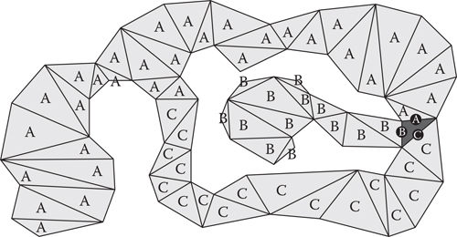
Figure 22.4
The result of a Dijkstra floodfill starting from the black node. Each node during the Dijkstra search is marked with the starting edge on the optimal path back to the starting node.
In a Dijkstra search, this starting node edge is normally not recorded, but now we need to store this information. Every node’s data structure needs to contain a new value representing this starting node edge. During the Dijkstra search, when the neighbors of a node are explored, the starting node edge is passed down to the neighboring nodes as they are placed on the open list. This transfers the starting node edge information from node to node during the search.
Once the Dijkstra floodfill has completed, every node is marked with a starting node edge. In the case of Figure 22.4, each node is marked with either an A, B, or C. The final task is to iterate through all nodes in the map and build up the bounding boxes that contain each starting node edge, as shown in Figure 22.5. Once complete, each bounding box (4 values representing left, right, top, and bottom) is stored on the appropriate starting node’s edge. This is the data that are used during runtime to prune the search during the goal-bounding check.
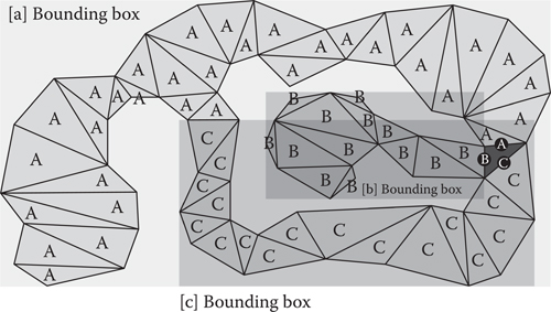
Figure 22.5
All nodes are iterated through to determine each bounding box for each starting edge.
In order to evaluate the effectiveness of goal bounding, we applied the algorithm to a similar setup as the Grid-Based Path Planning Competition (Sturtevant 2014), a competition that has run since 2012 for the purpose of comparing different approaches to grid-based path planning. All experiments were performed on maps from the GPPC competition and the Moving AI map repository (Sturtevant 2012). This includes maps from StarCraft, Warcraft III, and Dragon Age. We ran our code on a 2.4 GHz Intel Xeon E5620 with 12 GB of RAM.
Table 22.1 shows the comparison between a highly optimized A* solution, the same A* solution with goal bounding, JPS+, and JPS+ with goal bounding. The A* solution with goal bounding was 8.2 times faster than A* by itself. The JPS+ solution with goal bounding was 7.2 times faster than JPS+.
22.5.1 Applying Goal Bounding to JPS+
As shown in Table 22.1, JPS+ is an algorithm that can dramatically speed up pathfinding compared with A*, however it only works on uniform cost grids (where the cost between nodes must be consistent). JPS+ is a variant of A* that achieves its speed from pruning nodes from the search space, similar to goal bounding. However, JPS+ and goal bounding work in complementary ways so that combined effect is to speed up pathfinding by ~1500 times over A*. Although it is outside the scope of this chapter to explain JPS+ with goal bounding, there are two good resources if you wish to implement it (Rabin 2015, Rabin and Sturtevant 2016).
22.6 Similarities to Previous Algorithms
At its core, goal bounding is an approximation of the Floyd–Warshall all-pairs shortest paths algorithm. In Floyd–Warshall, the path between every single pair of nodes is precomputed and stored in a look-up table. Using Floyd–Warshall at runtime, no search algorithm is run, because the optimal path is simply looked up. This requires an enormous amount of data, which is O(n2) in the number of nodes. This amount of data is impractical for most games. For example, a StarCraft map of roughly 1000 × 1000 nodes would require about four terabytes.
As goal bounding is an approximation of Floyd–Warshall, it does not require nearly as much data. However, as mentioned previously in Section 22.1.1, it does require 32 values per node on a grid search space and 12 values per node on a navmesh search space (assuming triangular nodes). A StarCraft map of roughly 1000 × 1000 nodes would require about 60 MB of goal bounding data. Luckily, modern games using a navmesh might only have about 4000 total nodes for a level, which would require less than 100 KB of goal-bounding data.
Table 22.1 Comparison of Search Algorithm Speeds
Algorithm | Time (ms) | A* Factor |
A* | 15.492 | 1.0 |
A* with goal bounding | 1.888 | 8.2 |
JPS+ | 0.072 | 215.2 |
JPS+ with goal bounding | 0.010 | 1549.2 |
The goal-bounding algorithm was first introduced as an optimization to Dijkstra on road networks in 2005 and at the time was called geometric containers (Wagner et al. 2005). In 2014, Rabin independently reinvented geometric containers for use with A* and JPS+, introducing it as goal bounding to a GDC audience (Rabin 2015). Due to this history, it would be appropriate to refer to the algorithm as either geometric containers (Wagner et al. 2005), goal bounding (Rabin 2015), or simply as bounding boxes (Rabin and Sturtevant 2016).
For games that meet the constraints, goal bounding can speed up pathfinding dramatically–by nearly an order of magnitude. Not only can goal bounding be applied to any search algorithm on any type of search space, it can also be applied with other optimizations, such as hierarchical pathfinding, overestimating the heuristic, or open list optimizations (Rabin and Sturtevant 2013).
Rabin, S. 2015. JPS+ now with Goal Bounding: Over 1000 × Faster than A*, GDC 2015. http://www.gameaipro.com/Rabin_AISummitGDC2015_JPSPlusGoalBounding.zip (accessed February 12, 2017).
Rabin, S., and Sturtevant, N. R. 2013. Pathfinding optimizations. In Game AI Pro, ed. S. Rabin. Boca Raton, FL: CRC Press.
Rabin, S., and Sturtevant, N. R. 2016. Combining Bounding Boxes and JPS to Prune Grid Pathfinding, AAAI’16 Proceedings of the Thirtieth AAAI Conference on Artificial Intelligence. Phoenix, AZ: AAAI.
Sturtevant, N. R. 2012. Benchmarks for grid-based pathfinding. Transactions on Computational Intelligence and AI in Games, 4(2), 144–148.
Sturtevant, N. R. 2014. The grid-based path-planning competition. AI Magazine, 35(3), 66–68.
Sturtevant, N. R., and Rabin, S. 2017. Faster Dijkstra search on uniform cost grids. In Game AI Pro 3, ed. S. Rabin. Boca Raton, FL: CRC Press.
Wagner, D., Willhalm, T., and Zaroliagis, C. D. 2005. Geometric containers for efficient shortest-path computation. ACM Journal of Experimental Algorithmics, 10.