
Faster Dijkstra Search on Uniform Cost Grids
Dijkstra search is commonly used for single-source shortest path computations, which can provide valuable information about distances between states for many purposes in games, such as heuristics (Rabin and Sturtevant 2013), influence maps, or other analysis. In this chapter, we describe how we borrowed recent ideas from Jump Point Search (JPS) (Harabor and Grastien 2011) to significantly speed up Dijkstra search on uniform cost grids. We call this new algorithm Canonical Dijkstra. Although the algorithm has been described before (Sturtevant and Rabin 2016), this chapter provides more detail and examples of how the algorithms work in practice. This is just one example of how the ideas of JPS can be applied more broadly; we hope this will become a valuable part of your library of approaches. Note that the chapter does assume that the reader is familiar with how A* works.
23.2 Decomposing Jump Point Search
As Canonical Dijkstra builds on the ideas of JPS, we will describe the key ideas from JPS first. JPS has been described elsewhere in this book series (Rabin and Silva 2015). We describe it here in a slightly different manner (following Sturtevant and Rabin 2016) that will greatly simplify our presentation of Canonical Dijkstra.
23.2.1 Canonical Ordering of Paths
One of the problems with search on grids is that there are many duplicate paths between states. While A* will find these duplicates and avoid putting duplicates on the open list, it is costly to do so, because we still generate all of these states during the search and must look them up to detect that they are duplicates. It would be better if we could never generate the duplicates in the first place.
We can do this in two steps. In the first step, we generate a basic canonical ordering. A canonical ordering is a way of choosing which optimal path we prefer among all possible optimal paths. In Figure 23.1, we show a small map that has three possible optimal paths between the start and the goal. We define the canonical path as the path that has all diagonal moves before cardinal moves. It is more efficient to only generate the canonical path(s) and never generate any other paths.
We can generate states according to the canonical ordering directly (without comparing optimal paths) by limiting the successors of each state according to the parent. If the current state was reached by a diagonal action, then we allow three legal moves from the child: (1) the same diagonal action that was used to reach the state and (2 and 3) the two cardinal components of the same diagonal action. If a cardinal action (N/S/E/W) was used to reach a state, the only legal move is to move in the same direction. In the canonical ordering, we always take diagonal actions before cardinal actions, so once a cardinal action is part of a path, all remaining actions must also be cardinal actions.
We illustrate this in part (a) on the left of Figure 23.2, where the start state is marked with an “S” and lines label the canonical paths. Each state that is reached is reached optimally by a single path, and no duplicates will be generated. But, we also notice that not all states in the map are reached. In particular, there are obstacles that block some canonical paths. Luckily, we can fix this problem when generating the canonical ordering.
Suppose the search is currently moving north. Normally the search would continue north until an obstacle was reached and then would stop. But now, we need to do one additional check. If the search passes on obstacle to the east, which then ends, it knows that the basic canonical ordering will not reach this state. So, we need to reset the canonical ordering to allow it to reach states that are blocked by obstacles. We illustrate this in part (b) on the right of Figure 23.2. The black dots are the places where the canonical ordering was restarted (once again allowing diagonal moves) after passing obstacles. These dots are called jump points.
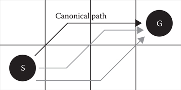
Figure 23.1
The canonical path (top) has diagonal actions before cardinal actions, unlike the noncanonical paths (in gray).
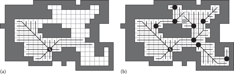
Figure 23.2
(a) The basic canonical ordering starting from the state marked S. (b) The full canonical ordering, including jump points (black circles).
Using jump points guarantees that every state in the map will be reached. While the number of duplicate paths is greatly reduced, because we only generate successors along the black lines, there still can be duplicates such as the one jump point in gray. This jump point can be reached from two different directions. Search is needed to resolve the optimal path lengths in this region of the map.
23.2.2 JPS and Canonical Orderings
We can now describe JPS in terms of the canonical ordering. The basic version of JPS does no preprocessing on the map before search. At runtime, it starts at the start state and generates a basic canonical ordering. All states visited when generating the canonical ordering are immediately discarded with the exception of jump points and the goal state, which are placed in the open list. It then chooses the best state from the open list to expand next. If this state is the goal, it terminates. Otherwise, it generates the canonical ordering from this new state, putting any new jump points or the goal into the open list. This process continues until the goal is found. It is possible that a jump point can be reached from two different directions, which is why jump points need to be placed in the open list. This ensures that a jump point is not expanded until it is reached with the optimal path.
JPS can be seen as searching on an abstract graph defined by the jump points and the goal in the graph. These are the only states that are put into the open list. But, because it has not preprocessed the map, it still has to scan the map to find the jump points and the goal. Scanning the map is far faster than putting all of these states into the open list, so JPS is usually faster than a regular A* search. Note, however, that JPS might scan more of the map than is necessary. So, in large, wide open spaces JPS can have a significant overhead. Given this understanding of JPS, we can now describe Canonical Dijkstra.
Canonical Dijkstra is, in many ways, similar to JPS. It uses the canonical ordering to generate states and searches over jump points. But, while JPS only puts jump points and the goal into the open and closed lists, Canonical Dijkstra needs to record the distance to every state in the state space in the closed list. Thus, Canonical Dijkstra must write the g-cost of every state that it visits (not just the jump points) into the closed list. This is where Canonical Dijkstra saves over a regular Dijkstra search–Dijkstra’s algorithm would put all of these states into the open list before expanding them and writing their costs to the closed list. Canonical Dijkstra writes these values directly to the closed list.
We show the first step of Canonical Dijkstra in Figure 23.3, but now we label the g-cost of each state as it is filled in by the search. In this example, diagonals have cost 1.5. To begin (part (a) on the left), the start is in open with cost 0.0. When the start state is expanded (part (b) on the right), the canonical ordering is generated, and the g-cost of every state visited is filled in a single step. Three jump points are reached, which are added to the open list; these states are marked with circles. This process continues until all states are reached by the search.
The most interesting step is shown in Figure 23.4. Here we see what happens when the search reaches the same state from different directions. The next state to be expanded (part (a) on the left) has cost 11.0 and is found at the top of the map. This state can reach its N, NE, and E neighbors with shorter path cost than they were previously reached. So, the g-costs are updated (part (b) on the right) after the node is expanded. One of these states (with g-cost 14.0 in the top side of the figure) was not previously a jump point. But, when reached from this direction, this state is a jump point. So, the state must be removed from the closed list and put onto the open list for further expansion.
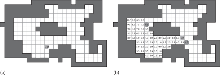
Figure 23.3
The first step of Canonical Dijkstra. Initially, (a) the start state is in the open list with cost 0. After the first expansion step, (b) the canonical ordering is followed until jump points are reached, and all visited states are labeled with their g-costs.
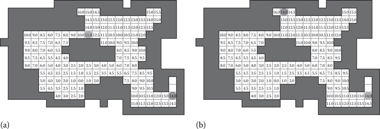
Figure 23.4
(a) In this step, Canonical Dijkstra expands the state at the top, finding a shorter path to several states nearby that have already been visited. (b) The search also finds a state that was not previously a jump point, but when reached from the new path is now a jump point.
Pseudocode for the Canonical Dijkstra algorithm can be found in Listing 23.1. The main procedure is a best-first search that repeatedly removes the best state from the open list. The canonical ordering code is the meat of the algorithm. While generating the canonical ordering, it keeps track of the current g-cost. As long as the canonical ordering finds a shorter cost path to a given state, the g-costs for that state are written directly into the closed list. When the canonical ordering generates a state with equal or larger g-cost than the copy in the open list, the process stops. When the canonical ordering finds a jump point, it adds that jump point to the open list. Since there is no goal, we do not have to check for the goal.
Listing 23.1. Canonical Dijkstra pseudocode.
CanonicalDijkstra(start)
{
initialize all states to be in closed with cost ∞
place start in open with cost 0
while (open not empty)
remove best from open
CanonicalOrdering(best, parent of best, 0)
}
CanonicalOrdering(child, parent, cost)
{
if (child in closed)
if (cost of child in closed > cost)
update cost of child in closed
else
return
if (child is jump point)
if on closed, remove from closed
update parent // for canonical ordering
add child to open with cost
else if (action from parent to child is diagonal d)
next = Apply(d, child)
CanonicalOrdering(next, child, cost + diagonal)
next = Apply(first cardinal in d, child)
CanonicalOrdering(next, child, cost + cardinal)
next = Apply(second cardinal in d, child)
CanonicalOrdering(next, child, cost + cardinal)
else if (action from parent to child is cardinal c)
next = Apply(c, child)
CanonicalOrdering(next, child, cost + cardinal)
}
23.3.1 Performance
The performance of Canonical Dijkstra depends on the type of map used. In random maps, there are many jump points, so the savings are lesser than on maps with larger open areas, where many g-costs can be written very quickly, bypassing the open list. We found 2.5× speedup on random maps and a 4.0× speedup on maps from StarCraft. These savings were independent of whether the base implementation was standard or high performance.
This chapter shows that JPS is using a canonical ordering to avoid duplicates during search. It borrows the idea of the canonical ordering to build an improved version of Dijkstra search that can perform single-source shortest path computations more efficiently by avoiding putting too many states into the open list.
Harabor, D. and Grastien, A. 2011. Online graph pruning for pathfinding on grid maps. In Proceedings of the Twenty-Fifth {AAAI} Conference on Artificial Intelligence. San Francisco, CA, pp. 1114–1119.
Rabin, S. and Sturtevant, N. R. 2013. Pathfinding architecture optimizations. In Game AI Pro, ed S. Rabin. Boca Raton, FL: CRC Press, pp. 241–252. http://www.gameaipro.com/GameAIPro/GameAIPro_Chapter17_Pathfinding_Architecture_Optimizations.pdf.
Rabin, S. and Silva, F. 2015. JPS+: An extreme A* speed optimization for static uniform cost grids. In Game AI Pro 2, ed. S. Rabin. Boca Raton, FL: CRC Press, pp. 131–143.
Sturtevant, N. R. and Rabin, S. 2016. Canonical Orderings on Grids, International Joint Conference on Artificial Intelligence (IJCAI), pp. 683–689. http://web.cs.du.edu/~sturtevant/papers/SturtevantRabin16.pdf.