25

Combat Outcome Prediction for Real-Time Strategy Games

Marius Stanescu, Nicolas A. Barriga, and Michael Buro

25.1  Introduction

Smart decision-making at the tactical level is important for AI agents to perform well in real-time strategy (RTS) games, in which winning battles is crucial. Although human players can decide when and how to attack based on their experience, it is challenging for AI agents to estimate combat outcomes accurately. Prediction by running simulations is a popular method, but it uses significant computational resources and needs explicit opponent modeling in order to adjust to different opponents.

This chapter describes an outcome evaluation model based on Lanchester’s attrition laws, which were introduced in Lanchester’s seminal book Aircraft in Warfare: The Dawn of the Fourth Arm in 1916 (Lanchester 1916). The original model has several limitations that we have addressed in order to extend it to RTS games (Stanescu et al. 2015). Our new model takes into account that armies can be comprised of different unit types, and that troops can enter battles with any fraction of their maximum health. The model parameters can easily be estimated from past recorded battles using logistic regression. Predicting combat outcomes with this method is accurate, and orders of magnitude are faster than running combat simulations. Furthermore, the learning process does not require expert knowledge about the game or extra coding effort in case of future unit changes (e.g., game patches).

25.2  The Engagement Decision

Suppose you command 20 knights and 40 swordsmen and just scouted an enemy army of 60 bowmen and 40 spearmen. Is this a fight you can win, or should you avoid the battle and request reinforcements? This is called the engagement decision (Wetzel 2008).

25.2.1  Scripted Behavior

Scripted behavior is a common choice for making such decisions, due to the ease of implementation and very fast execution. Scripts can be tailored to any game or situation. For example, always attack is a common policy for RPG or FPS games–for example, guards charging as soon as they spot the player. More complex strategy games require more complicated scripts: attack closest, prioritize wounded, attack if enemy does not have cavalry, attack if we have more troops than the enemy, or retreat otherwise. AI agents should be able to deal with all possible scenarios encountered, some of which might not be foreseen by the AI designer. Moreover, covering a very wide range of scenarios requires a significant amount of development effort.

There is a distinction we need to make. Scripts are mostly used to make decisions, while in this chapter we focus on estimating the outcome of a battle. In RTS games, this prediction is arguably the most important factor for making decisions, and here we focus on providing accurate information to the AI agent. We are not concerned with making a decision based on this prediction. Is losing 80% of the initial army too costly a victory? Should we retreat and potentially let the enemy capture our castle? We leave these decisions to a higher level AI and focus on providing accurate and useful combat outcome predictions. Examples about how these estimations can improve decision-making can be found in Bakkes and Spronck (2008) and Barriga et al. (2017).

25.2.2  Simulations

One choice that bypasses the need for extensive game knowledge and coding effort is to simulate the battle multiple times, without actually attacking in the game, and to record the outcomes. If from 100 mock battles we win 73, we can estimate that the chance of winning the engagement is close to 73%. For this method to work, we need the combat engine to allow the AI system to simulate battles. Moreover, it can be difficult to emulate enemy player behaviors, and simulating exhaustively all possibilities is often too costly.

Technically, simulations do not directly predict the winner but provide information about potential states of the world after a set of actions. Performing a playout for a limited number of simulation frames is faster, but because there will often not be a clear winner, we need a way of evaluating our chances of winning the battle from the resulting game state. Evaluation (or scoring) functions are commonly employed by look-ahead algorithms, which forward the current state using different choices and then need to numerically compare the results. Even if we do not use a search algorithm, or partial simulations, an evaluation function can be called on the current state and help us make a decision based on the predicted combat outcome. However, accurately predicting the result of a battle is often a difficult task.

The possibility of equal (or nearly equal armies) fighting with the winner seeing the battle through with a surprisingly large remaining force is one of the interesting aspects of strategic, war simulation-based games. Let us consider two identical forces of 1000 men each; the Red force is divided into two units of 500 men, which serially engage the single (1000 men) Blue force. Most linear scoring functions, or a casual gamer, would identify this engagement as a slight win for the undivided Blue army, severely underestimating the “concentration of power” axiom of war. A more experienced armchair general would never make such a foolish attack, and according to the Quadratic Lanchester model (introduced below), the Blue force completely destroys the Red army with only moderate loss (i.e., 30%) to itself.

25.3  Lanchester’s Attrition Models

The original Lanchester equations represent simplified combat models: each side has identical soldiers and a fixed strength (i.e., there are no reinforcements), which governs the proportion of enemy soldiers killed. Range, terrain, movement, and all other factors that might influence the fight are either abstracted within the parameters or ignored entirely. Fights continue until the complete destruction of one force, and as such the following equations are only valid until one of the army sizes is reduced to 0. The general form of the attrition differential equations is:

$\frac{dA}{dt}=-\text{β}{A}^{2-n}B\text{and}\frac{dB}{dt}=-\text{α}{B}^{2-n}A$

(25.1)

where:

t denotes time

A, B are force strengths (number of units) of the two armies assumed to be functions of time

By removing time as a variable, the pair of differential equations can be combined into $\text{α}\text{(}{A}^n-A_0^n\text{)}=\text{β}\text{(}{B}^n-B_0^n\text{)}.$

Parameters α and β are attrition rate coefficients representing how fast a soldier in one army can kill a soldier in the other. The equation is easier to understand if one thinks of β as the relative strength of soldiers in army B; it influences how fast army A is reduced. The exponent n is called the attrition order and represents the advantage of a higher rate of target acquisition. It applies to the size of the forces involved in combat but not to the fighting effectiveness of the forces which is modeled by attrition coefficients α and β. The higher the attrition order, the faster any advantage an army might have in combat effectiveness is overcome by numeric superiority.

For example, choosing n = 1 leads to $\text{α}\text{(}A-A_0)=\text{β}\text{(}B-B_0)$, which is known as Lanchester’s Linear Law. This equation models situations in which one soldier can only fight a single soldier at a time. If one side has more soldiers, some of them will not always be fighting as they wait for an opportunity to attack. In this setting, the casualties suffered by both sides are proportional to the number of fighters and the attrition rates. If α = β, then the above example of splitting a force into two and fighting the enemy sequentially will have the same outcome as without splitting: a draw. This was originally called Lanchester’s Law of Ancient Warfare, because it is a good model for battles fought with melee weapons (such as spears or swords, which were the common choices of Greek or Roman soldiers).

Choosing n = 2 results in the Square Law, which is also known as Lanchester’s Law of Modern Warfare. It is intended to apply to ranged combat, as it quantifies the value of the relative advantage of having a larger army. However, the Squared Law has nothing to do with range–what is really important is the rate of acquiring new targets. Having ranged weapons generally lets soldiers engage targets as fast as they can shoot, but with a sword or a pike, one would have to first locate a target and then move to engage it. In our experiments for RTS games that have a mix of melee and ranged units, we found attrition order values somewhere in between working best. For our particular game–StarCraft Broodwar–it was close to 1.56.

The state solution for the general law can be rewritten as $\text{α}{A}^n-\text{β}{B}^n=\text{α}{A}_0^n-\text{β}{B}_0^n=k$. Constant k depends only on the initial army sizes A₀ and B₀. Hence, if $k>0$ or equivalently $\text{α}{A}_0^n>\text{β}{B}_0^n$, then player A wins. If we denote the final army sizes with $A_f\text{and}{B}_f$ and assume player B lost, then $B_f=0$ and $\text{α}{A}_0^n-\text{β}{B}_0^n=\text{α}{A}_f^n-0$, and we can predict the remaining victorious army size $A_f$. We just need to choose appropriate values α and β that reflect the strength of the two armies, a task we will focus on in the next section.

25.4  Lanchester Model Parameters

In RTS games, it is often the case that both armies are composed of various units, with different capabilities. To model these heterogeneous army compositions, we need to replace the army effectiveness with an average value

${\text{α}}_{\text{avg}}=\frac{{\sum }_{j=1}^A{\text{α}}_j}{A}$

(25.2)

where:

α_j is the effectiveness of a single unit

A is the total number of units

We can see that predicting battle outcomes will require strength estimates for each unit involved. In the next subsections, we describe how these parameters can be either manually created or learned.

25.4.1  Choosing Strength Values

The quickest and easiest way of approximating strength is to pick a single attribute that you feel is representative. For instance, we can pick α_i = level_i if we think that a level k dragon is k times as strong as a level 1 footman. Or maybe a dragon is much stronger, and if we choose ${\text{α}}_i=5^{{\text{level}}_i}$ instead, then it would be equivalent to 5^k footmen.

More generally, we can combine any number of attributes. For example, the cost of producing or training a unit is very likely to reflect unit strength. In addition, if we would like to take into account that injured units are less effective, we could add the current and maximum health points to our formula:

${\text{α}}_i=\frac{\text{Cost}\left(i\right)\text{HP}\left(i\right)}{\text{MaxHP}\left(i\right)}$

(25.3)

This estimate may work well, but using more attributes such as attack or defense values, damage, armor, or movement speed could improve prediction quality, still. We can create a function that takes all these attributes as parameters and outputs a single value. However, this requires a significant understanding of the game, and, moreover, it will take a designer a fair amount of time to write down and tune such an equation.

Rather than using a formula based on attack, health, and so on, it is easier to pick some artificial values: for instance, the dragon may be worth 100 points and a footman may worth just one point. We have complete control over the relative combat values, and we can easily express if we feel that a knight is five times stronger than a footman. The disadvantage is that we might guess wrong, and thus we still have to playtest and tune these values. Moreover, with any change in the game, we need to manually revise all the values.

25.4.2  Learning Strength Values

So far, we have discussed choosing unit strength values for our combat predictor via two methods. First, we could produce and use a simple formula based on one or more relevant attributes such as unit level, cost, health, and so on. Second, we could directly pick a value for each unit type based mainly on our intuition and understanding of the game. Both methods rely heavily on the designer’s experience and on extensive playtesting for tuning. To reduce this effort, we can try to automatically learn these values by analyzing human game replays or, alternatively, letting a few AI systems play against each other.

Although playtesting might ensure that AI agents play well versus the game designers, it does not guarantee that the agents will also play well against other unpredictable players. However, we can adapt the AI to any specific player by learning a unique set of unit strength values taking into account only games played by this player. For example, the game client can generate a new set of AI parameters before every new game, based on a number of recent battles. Automatically learning the strength values will require less designer effort and provide better experiences for the players.

The learning process can potentially be complex, depending on the machine learning tools to be used. However even a simple approach, such as logistic regression, can work very well, and it has the advantage of being easy to implement. We will outline the basic steps for this process here.

First, we need a dataset consisting of as many battles as possible. Some learning techniques can provide good results after as few as 10 battles (Stanescu et al. 2013), but for logistic regression, we recommend using at least a few hundred. If a player has only fought a few battles, we can augment his dataset with a random set of battles from other players. These will be slowly replaced by “real” data as our player fights more battles. This way the parameter estimates will be more stable, and the more the player plays, the better we can estimate the outcome of his or her battles.

An example dataset is shown in Table 25.1. Each row corresponds to one battle, and we will now describe what each column represents. If we are playing a game with only two types of soldiers, armed with spears or bows, we need to learn two parameters for each player: $w_{\text{spear}}$ and $w_{\text{bow}}$. To maintain sensitivity to unit injuries, we use ${\text{α}}_j=w_{\text{spear}}\text{HP(}\text{}\text{}\text{}j\text{)}$ or ${\text{α}}_j=w_{\text{bow}}\text{HP(}\text{}\text{}\text{}j\text{)}$, depending on unit type. The total value of army A can then be expressed as:

$$\begin{gathered} L\text{(}\text{}\text{}\text{}A\text{)}={\text{α}}_{\text{avg}}{A}^n=A^{n-1}\sum _{j=1}^A{\text{α}}_j=A^{n-1}\sum _{j=1}^A{w}_j\text{HP(}\text{}\text{}\text{}j\text{)} \\ =A^{n-1}(w_{\text{spear}}H{P}_s+w_{\text{bow}}{\text{HP}}_b) \end{gathered}$$

(25.4)

HP_s is the sum of the health points of all of player A’s spearmen. After learning all w parameters, the combat outcome can be estimated by subtracting L(A)–L(B). For simplicity, in Table 25.1, we assume each soldier’s health is a number between 0 and 1.

25.4.3  Learning with Logistic Regression

As a brief reminder, logistic regression uses a linear combination of variables. The result is squashed through the logistic function F, restricting the output to (0,1), which can be interpreted as the probability of the first player winning.

$y=a_0+a_1{X}_1+a_2{X}_2+\cdots F\left(y\right)=\frac{1}{1+e^{-y}}$

(25.5)

For example, if v = 0, then F = 0.5 which is a draw. If v > 0, then the first player has the advantage. For ease of implementation, we can process the previous table in such a way that each column is associated with one parameter to learn, and the last column contains the battle outcomes (Table 25.2). Let us assume that both players are equally adept at controlling spearmen, but bowmen require more skill to use efficiently and their strength value could differ when controlled by the two players:

$$\begin{gathered} y=L\left(A\right)-L\left(B\right) \\ =w_{\text{spear}}\left(A^{n-1}{\text{HP}}_{sA}-B^{n-1}{\text{HP}}_{sB}\right)+w_{\text{bow}A}\left(A^{n-1}{\text{HP}}_{bA}\right)-w_{\text{bow}B}\left(B^{n-1}{\text{HP}}_{bB}\right) \end{gathered}$$

(25.6)

This table can be easily used to fit a logistic regression model in your coding language of choice. For instance, using Python’s pandas library, this can be done in as few as five lines of code.

Table 25.1 Example Dataset Needed for Learning Strength Values

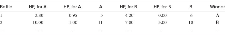
Table 25.2 Processed Dataset (All But Last Column Correspond to Parameters to be Learned)

$A^{n-1}\text{H}{\text{P}}_{sA}-B^{n-1}\text{H}{\text{P}}_{sB}$	$A^{n-1}\text{H}{\text{P}}_{bA}$	$-(B^{n-1}\text{H}{\text{P}}_{bB})$	Winner
…	…	…	…

25.5  Experiments

We have used the proposed Lanchester model but with a slightly more complex learning algorithm in UAlbertaBot, a StarCraft open-source bot for which detailed documentation is available online (UAlbertaBot 2016). The bot runs combat simulations to decide if it should attack the opponent with the currently available units if a win is predicted or retreat otherwise. We replaced the simulation call in this decision procedure with a Lanchester model-based prediction.

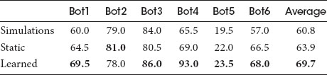
Three tournaments were run. First, our bot ran one simulation with each side using an attack closest policy. Second, it used the Lanchester model described here with static strength values for each unit based on its damage per frame and current health: α_i = DMG(i)HP(i). For the last tournament, a set of strength values was learned for each of 6 match-ups from the first 500 battles of the second tournament. In each tournament, 200 matches were played against 6 top bots from the 2014 AIIDE StarCraft AI tournament. The results–winning percentages for different versions of our bot–are shown in Table 25.3. On average, the learned parameters perform better than both static values and simulations, but be warned that learning without any additional hand checks might lead to unexpected behavior such as the match against Bot2 where the win rate actually drops by 3%.

Our bot’s strategy is very simple: it only trains basic melee units and tries to rush the opponent and keep the pressure up. This is why we did not expect very large improvements from using Lanchester models, as the only decision they affect is whether to attack or to retreat. More often than not this translates into waiting for an extra unit, attacking with one unit less, and better retreat triggers. Although this makes all the difference in some games, using this accurate prediction model to choose the army composition, for example, could lead to much bigger improvements.

25.6  Conclusions

In this chapter, we have described an approach to automatically generate an effective combat outcome predictor that can be used in war simulation strategy games. Its parameters can be static, fixed by the designer, or learned from past battles. The choice of training data provided to the algorithm ensures adaptability to specific opponents or maps. For example, learning only from siege battles will provide a good estimator for attacking or defending castles, but it will be less precise for fighting in large unobstructed areas where cavalry might prove more useful than, say, artillery. Using a portfolio of estimators is an option worth considering.

Table 25.3 Our Bot’s Winning % Using Different Methods for Combat Outcome Prediction

Adaptive game AI can use our model to evaluate newly generated behaviors or to rank high-level game plans according to their chances of military success. As the model parameters can be learned from past scenarios, the evaluation will be more objective and stable to unforeseen circumstances when compared to functions created manually by a game designer. Moreover, learning can be controlled through the selection of training data, and it is very easy to generate map- or player-dependent parameters. For example, one set of parameters can be used for all naval battles, and another set can be used for siege battles against the elves. However for good results, we advise acquiring as many battles as possible, preferably tens or hundreds.

Other use cases for accurate combat prediction models worth considering include game balancing and testing. For example, if a certain unit type is scarcely being used, it can help us decide if we should boost one of its attributes or reduce its cost as an extra incentive for players to use it.

References

Bakkes, S. and Spronck, P., 2008. Automatically generating score functions for strategy games. In Game AI Programming Wisdom 4, ed. S. Rabin. Hingham, MA: Charles River Media, pp. 647–658.

Barriga, N., Stanescu, M., and Buro, M., 2017. Combining scripted behavior with game tree search for stronger, more robust game AI. In Game AI Pro 3: Collected Wisdom of Game AI Professionals, ed. S. Rabin. Boca Raton, FL: CRC Press.

Lanchester, F.W., 1916. Aircraft in Warfare: The Dawn of the Fourth Arm. London: Constable limited.

Stanescu, M., Hernandez, S.P., Erickson, G., Greiner, R., and Buro, M., 2013. October. Predicting army combat outcomes in StarCraft. In Ninth Annual AAAI Conference on Artificial Intelligence and Interactive Digital Entertainment (AIIDE), October 14–18, 2013. Boston, MA.

Stanescu, M., Barriga, N., and Buro, M., 2015, September. Using Lanchester attrition laws for combat prediction in StarCraft. In Eleventh AIIDE Conference, November 14–18, 2015. Santa Cruz, CA.

UAlbertaBot github repository, maintained by David Churchill., 2016. https://github.com/davechurchill/ualbertabot.

Wetzel, B., 2008. The engagement decision. In Game AI Programming Wisdom 4, ed. S. Rabin. Boston, MA: Charles River Media, pp. 443–454.