26
Introduction to SQL
Eventually, you (or someone else) must build the database that you've designed. Also at some point, someone will probably want to actually use the database you've spent so much time designing.
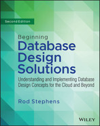
Structured Query Language (SQL, sometimes pronounced “sequel”) is a database language that includes commands that let you build, modify, and manipulate relational databases. Many database tools use SQL either directly or behind the scenes to create and manipulate the database. For example, Figure 26.1 shows how the pgAdmin tool uses SQL to define the order_items table used in Chapters 18 and 19, which cover PostgreSQL.
Because SQL is standardized, many database management tools use it to control relational databases. They use buttons, drop-down menus, check boxes, and other user interface controls to let you design a database interactively, and then they send SQL code to the database engine to do the work.
In addition to using database tools to generate your SQL code, you can write that code yourself, which lets you create and modify the database as needed. It also lets you add data to put the database in a known state for testing. In fact, SQL is so useful for building databases that it's the topic of the next chapter.
SQL is such an important part of database development that your education as a database designer is sadly lacking if you don't at least understand the basics. (The other developers will rightfully mock you if you don't chuckle when you see a T-shirt that says, “SELECT * FROM People WHERE NOT Clue IS null.”)
In this chapter, you'll learn how to use SQL to do the following:
- Create and delete tables.
- Insert data into tables.
- Select data from the database using various criteria and sort the results.
- Modify data in the database.
- Delete records.
BACKGROUND
SQL was developed by IBM in the mid-1970s. It is an English-like command language for building and manipulating relational databases.
From a small but ambitious beginning, SQL has grown into a large language containing about 70 commands with hundreds of variations. Because SQL has grown so large, I cannot possibly cover every nook and cranny. Instead, this chapter gives a brief introduction to SQL and then describes some of the most useful SQL commands in greater detail. Even then, this chapter doesn't have room to cover most of the more interesting commands completely. The SELECT statement alone includes so many variations that you could practically write a book about just that one command.
FINDING MORE INFORMATION
SQL is intuitive enough that, once you master the basics, you should be able to get pretty far on your own. The Internet is practically clogged with websites that are chock-full of SQL goodness in the form of tutorials, references, FAQs, question and answer forums, and discussion groups.
In fact, I'll start you off with a small list of websites right now. The following list shows a few websites that provide SQL tutorials:
https://sqlcourse.comhttps://sql.orghttps://sqltutorial.nethttps://sqltutorial.orghttps://tutorialspoint.com/sql/index.htmhttps://w3schools.com/sql
For help on specific issues, you should find a few SQL forums where you can ask questions. An enormous number of developers work with databases and SQL on a daily basis, so there are lots of forums out there. Just search for SQL forum to find more forums than you can shake a SELECT statement at.
Tutorials can help you get started using some of the more common SQL statements, but they aren't designed as references. If you need more information about a particular command, you should look for a SQL reference. At the following sites you'll find references for different versions of SQL:
- MariaDB—
https://mariadb.com/kb/en/sql-statements - Microsoft Transact-SQL—
https://learn.microsoft.com/en-us/sql/t-sql/language-reference - MySQL—
https://dev.mysql.com/doc/refman/8.0/en - Oracle SQL—
www.adp-gmbh.ch/ora/sql - PostgreSQL—
https://postgresql.org/docs/8.1/sql-commands.html
Each of these pages provides simple navigation to look up specific SQL commands.
Note, however, that these web pages deal with specific versions of SQL. Though the basics of any version of SQL are fairly standard, there are some differences between the various flavors.
STANDARDS
Although all relational databases support SQL, different databases may provide slightly different implementations. This is such an important point that I'll say it again.
Both the International Organization for Standardization (ISO) and the American National Standards Institute (ANSI) have standards for the SQL language, and most database products follow those standards pretty faithfully. However, different database products also add extra features to make certain chores easier. Those extras can be useful but only if you are aware of which features are standard and which are not, and you use the extra features with caution.
For example, in the Transact-SQL language used by SQL Server, the special values @@TOTAL_ERRORS, @@TOTAL_READS, and @@TOTAL_WRITES return the total number of disk write errors, disk reads, and disk writes, respectively, since SQL Server was last started. Other relational databases don't provide those, although they may have their own special values that return similar statistics.
If you use these kinds of special features haphazardly, it may be very hard to rebuild your database or the applications that use it if you are forced to move to a new kind of database. For that matter, extra features can make it hard for you to reuse tools and techniques that you develop in your next database project.
Fortunately, most flavors of SQL are 90 percent identical. You can guard against troublesome changes in the future by keeping the nonstandard features in a single code module or library as much as possible.
Usually the places where SQL implementations differ the most is in system-level chores such as database management and searching metadata. For example, different databases might provide different tools for searching through lists of tables, creating new databases, learning about the number of reads and writes that the database performed, examining errors, and optimizing queries.
MULTISTATEMENT COMMANDS
Many (but not all) databases allow you to execute multiple commands at once if you separate them with semicolons. Even then, some databases disable that capability by default. In that case, you need to take extra steps to enable this feature.
For example, the following code shows how a Python program can execute multistatement commands in MariaDB:
# Semi-colons.# Create the tables.import pymysqlfrom pymysql.connections import CLIENT# Connect to the database server.conn = pymysql.connect(host="localhost",user="root",password="G4eJuHFIhFOa13m",database="Chapter26Data",client_flag=CLIENT.MULTI_STATEMENTS)# Create a cursor.cur = conn.cursor()cur.execute("""DROP TABLE IF EXISTS Crewmembers;CREATE TABLE Crewmembers (FirstName VARCHAR(45) NOT NULL,LastName VARCHAR(45) NOT NULL);""")cur.execute("""INSERT INTO Crewmembers VALUES ("Malcolm", "Reynolds");INSERT INTO Crewmembers VALUES ('Hoban "Wash"', "Washburne");INSERT INTO Crewmembers VALUES ("Zoë", "Washburne");INSERT INTO Crewmembers VALUES ("Kaylee", "Frye");INSERT INTO Crewmembers VALUES ("Jayne", "Cobb");SELECT * FROM Crewmembers""")cur.execute("SELECT * FROM Crewmembers")rows = cur.fetchall()for row in rows:print(row[0] + " " + row[1])# Close the connection.conn.commit()conn.close()
This code first imports the pymysql and pymysql.connections.CLIENT modules. It then connects to the database. The code sets the connect method's client_flag parameter to CLIENT.MULTI_STATEMENTS to enable multistatement commands. The setup code finishes by creating a cursor to manipulate the database.
The program then executes a DROP TABLE statement and a CREATE TABLE statement in a single command. Notice how the commands are separated by semicolons. MariaDB is uncooperative if you leave out the semicolons. You can omit the semicolon after the final command if you like, but I've included it for consistency. (It also makes it easier to add more commands at the end of the sequence without forgetting to add new semicolons.)
Next, the code uses a multistatement command to execute five INSERT statements.
In both execute calls, the Python code uses the multiline string delimiter """ so the statements can include single or double quotes. The second INSERT statement uses single quotes around the first name value so that it can include embedded double quotes for Wash's nickname.
The opening and closing triple quotes are on the lines before and after the SQL code, so the SQL code is exactly as it would appear in a script.
After it inserts the records, the code executes a SELECT statement and displays the new records. The code finishes by committing the changes and closing the database connection.
The following shows the program's output:
Malcolm ReynoldsHoban "Wash" WashburneZoë WashburneKaylee FryeJayne Cobb
If you include a SELECT statement inside a multistatement command the fetchall method returns an empty result, so you should execute SELECT statements separately, at least in MariaDB.
BASIC SYNTAX
As is mentioned earlier in this chapter, SQL is an English-like language. It includes command words such as CREATE, INSERT, UPDATE, and DELETE.
SQL is case-insensitive. That means it doesn't care whether you spell the DELETE keyword as DELETE, delete, Delete, or DeLeTe.
SQL also doesn't care about the capitalization of database objects such as table and field names. If a database has a table containing people from the Administrative Data Organization, SQL doesn't care whether you spell the table's name ADOPEOPLE, AdoPeople, or aDOPEople. (Although the last one looks like “a dope ople,” which may make pronunciation tricky and might annoy your admins.)
To make the code easier to read, however, most developers write SQL command words in ALL CAPS and they write database object names using whatever capitalization they used when building the database. For example, I prefer MixedCase for table and field names.
Unfortunately, not all database products handle variations in capitalization in exactly the same way. For example, as you learned in Chapter 18, “PostgreSQL in Python,” PostgreSQL “helpfully” converts table and column names to lowercase. Run some tests to see whether you and your database have the same capitalization fashion sense, and then be prepared to do some rewriting if you're forced to switch databases.
A final SQL feature that makes commands easier to read is that SQL ignores whitespace. That means it ignores spaces, tabs, line feeds, and other “spacing” characters, so you can use those characters to break long commands across multiple lines or to align related statements in columns.
For example, the following code shows a typical SELECT command as I would write it:
SELECT FirstName, LastName, Clue,Street, City, State, ZipFROM PeopleWHERE NOT Clue IS NULLORDER BY Clue, LastName, FirstName
This command selects name and address information from the records in the People table where the record's Clue field has a value that is not null. (Basically, it selects people who have a clue, normally a pretty small data set.) It sorts the results by Clue, LastName, and FirstName.
This command places the different SQL clauses on separate lines to make them easier to read. It also places the person's name and address on separate lines and indents the address fields so they line up with the FirstName field. That makes it easier to pick out the SELECT, FROM, WHERE, and ORDER BY clauses.
COMMAND OVERVIEW
SQL commands are typically grouped into four categories: Data Definition Language (DDL), Data Manipulation Language (DML), Data Control Language (DCL), and Transaction Control Language (TCL).
Note that some commands have several variations. For example, in Transact-SQL the ALTER command has the versions ALTER DATABASE, ALTER FUNCTION, ALTER PROCEDURE, ALTER TABLE, ALTER TRIGGER, and ALTER VIEW. The following tables just provide an overview of the main function (ALTER) so you know where to look if you need one of these.
DDL commands define the database's structure. Table 26.1 briefly describes the most commonly used DDL commands.
TABLE 26.1: DDL commands
| COMMAND | PURPOSE |
|---|---|
ALTER | Modifies a database object such as a table, stored procedure, or view. The most important variation is ALTER TABLE, which lets you change a column definition or table constraint. |
CREATE | Creates objects such as tables, indexes, views, stored procedures, and triggers. In some versions of SQL, this also creates databases, users, and other high-level database objects. Two of the most important variations are CREATE TABLE and CREATE INDEX. |
DROP | Deletes database objects such as tables, functions, procedures, triggers, and views. Two of the most important variations are DROP TABLE and DROP INDEX. |
DML commands manipulate data. They let you perform the CRUD operations: Create, Read, Update, and Delete. (Where athletes “talk smack,” database developers “talk CRUD.”) Table 26.2 summarizes the most common DML commands. Generally developers think of only the CRUD commands INSERT, SELECT, UPDATE, and DELETE as DML commands, but this table includes cursor commands because they are used to select records.
TABLE 26.2: DML commands
| COMMAND | PURPOSE |
|---|---|
CLOSE | Closes a cursor. |
DECLARE | Declares a cursor that a program can use to fetch and process records a few at a time instead of all at once. |
DELETE | Deletes records from a table. |
FETCH | Uses a cursor to fetch rows. |
INSERT | Inserts new rows into a table. A variation lets you insert the result of a query into a table. |
SELECT | Selects data from the database, possibly saving the result into a table. |
TRUNCATE | Deletes all of the records from a table as a group without logging individual record deletions. It also removes empty space from the table while DELETE may leave empty space to hold data later. (Some consider TRUNCATE a DDL command, possibly because it removes empty space from the table. Or possibly just to be contrary. Or perhaps I'm the contrary one.) |
UPDATE | Changes the values in a record. |
DCL commands allow you control access to data. Depending on the database, you may be able to control user privileges at the database, table, view, or field level. Table 26.3 summarizes the two most common DCL commands.
TABLE 26.3: DCL commands
| COMMAND | PURPOSE |
|---|---|
GRANT | Grants privileges to a user |
REVOKE | Revokes privileges from a user |
TCL commands let you use transactions. A transaction is a set of commands that should be executed atomically as a single unit, so either every command is executed or none of the commands is executed.
For example, suppose you want to transfer money from one bank account to another. It would be bad if the system crashed after you subtracted money from the first account but before you added it to the other. If you put the two commands in a transaction, the database guarantees that either both happen or neither happens.
Table 26.4 summarizes the most common TCL commands.
TABLE 26.4: TCL commands
| COMMAND | PURPOSE |
|---|---|
BEGIN | Starts a transaction. Operations performed before the next COMMIT or ROLLBACK statement are part of the transaction. |
COMMIT | Closes a transaction, accepting its results. |
ROLLBACK | Rewinds a transaction's commands back to the beginning of the transaction or to a savepoint defined within the transaction. |
SAVE | Creates a savepoint within a transaction. (Transact-SQL calls this command SAVE TRANSACTION whereas PostgreSQL calls it SAVEPOINT.) |
The following sections describe the most commonly used commands in greater detail.
CREATE TABLE
The CREATE TABLE statement builds a database table. The basic syntax for creating a table is:
CREATE TABLE table_name (parameters)Here table_name is the name you want to give to the new table and parameters is a series of statements that define the table's columns. Optionally, parameters can include column-level and table-level constraints.
A column definition includes the column's name, its data type, and optional extras such as a default value or the keywords NULL or NOT NULL to indicate whether the column should allow null values.
A particularly useful option that you can add to the CREATE TABLE statement is IF NOT EXISTS. This clause makes the statement create the new table only if it doesn't already exist.
For example, the following statement creates a Students table with three fields. Notice how the code uses whitespace to make the field data types and NOT NULL clauses align so they are easier to read:
CREATE TABLE IF NOT EXISTS Students (StudentId INT NOT NULL AUTO_INCREMENT,FirstName VARCHAR(45) NOT NULL,LastName VARCHAR(45) NOT NULL,PRIMARY KEY (StudentId))
The StudentId field is an integer (INT) that is required (NOT NULL). The database automatically generates values for this field by adding 1 to the value it last generated (AUTO_INCREMENT).
The FirstName and LastName fields are required variable-length strings up to 45 characters long.
The table's primary key is the StudentId field.
A key part of a column's definitions is the data type. The following list summarizes the most common SQL data types:
BLOB—A Binary Large Object. This is any chunk of binary data such as a JPEG file, audio file, video file, or JSON document. The database knows nothing about the internal structure of this data so, for example, if the BLOB contains a JSON document the database cannot search its contents.BOOLEAN—A true or false value.CHAR—A fixed-length string. Use this for strings that always have the same length such as two-letter state abbreviations or five-digit ZIP Codes.DATE—A month, date, and year such as August 29, 1997.DATETIME—A date and time such as 2:14 a.m., August 29, 1997.DECIMAL(p, s)—A fixed-point number wherep(precision) gives the total number of digits ands(scale) gives the number of digits to the right of the decimal. For example,DECIMAL(6, 2)holds numbers of the form 1234.56.INT—An integer value.NUMBER—A floating-point number.TIME—A time without a date such as 2:14 a.m..TIMESTAMP—A date and time.VARCHAR—A variable-length string. Use this for strings of unknown lengths such as names and street addresses.
Specific database products often provide extra data types and aliases for these types. They also sometimes use these names for different purposes. For example, in different databases the INT data type might use 32 or 64 bits, and the database may provide other data types such as SMALLINT, TINYINT, BIGINT, and so forth to hold integers of different sizes.
Most databases can handle the basic data types but before you make specific assumptions (for example, that INT means 32-bit integer), check the documentation for your database product.
The following code builds a frankly hacked together table with the sole purpose of demonstrating most of the common data types. Notice that this command uses the combined FirstName and LastName fields as the table's primary key:
CREATE TABLE IF NOT EXISTS MishmashTable (FirstName VARCHAR(40) NOT NULL,LastName VARCHAR(40) NOT NULL,Age INT NULL,Birthdate DATE NULL,AppointmentDateTime DATETIME NULL,PreferredTime TIME NULL,TimeAppointmentCreated TIMESTAMP NULL,Salary DECIMAL(8,2) NULL,IncludeInvoice BOOLEAN NULL,Street VARCHAR(40) NULL,City VARCHAR(40) NULL,State CHAR(2) NULL,Zip CHAR(5) NULL,PRIMARY KEY (FirstName, LastName))
The following chapter has more to say about using the CREATE TABLE statement to build databases.
CREATE INDEX
The previous CREATE TABLE example uses INDEX clauses to define indexes for the table as it is being created. The CREATE INDEX statement adds an index to a table after the table has been created.
For example, the following statement adds an index named IDX_People_Names to the People table. This index makes it easier to search the table by using the records' combined FirstName/LastName fields:
CREATE INDEX IDX_People_Names ON People (FirstName, LastName)Some databases, such as PostgreSQL, don't let you create indexes inside a CREATE TABLE statement. In that case, you must use CREATE INDEX if you want the table to have an index. You can also use CREATE INDEX to add an index to a table if you didn't realize you would need one or you just forgot to do it earlier.
There's also sometimes a strategic reason to add the index after you create the table. Relational databases use complicated self-balancing trees to provide indexes. When you add or delete a record, the database must perform a nontrivial amount of work to update its index structures. If you add the records in sorted order, as is often the case when you first populate the database, this can mean even more work than usual because the tree structures tend to have trouble with sorted values so they perform a lot more work.
When you create an index after the table is populated, the database must perform a fair amount of work to build the index tree, but it has a big advantage that it doesn't when indexing records one at a time: it knows how many records are in the table. Instead of resizing the index tree as it is built one record at a time, the database can build a big empty tree, and then fill it with data.
Some databases may not use this information effectively, but some can fill the table and then add an index more quickly than they can fill the table if the index is created first. Note that the difference is small, so you probably shouldn't worry about creating the indexes separately unless you are loading a lot of records.
DROP
The DROP statement removes an object from the database. For example, the following statement removes the index named IDX_People_Names from the People table in a MariaDB database:
DROP INDEX IDX_People_Names ON PeopleThe following statement shows the Transact-SQL language version of the previous command:
DROP INDEX People.IDX_People_NamesThe following shows the PostgreSQL version:
DROP INDEX IDX_People_NamesThe other most useful DROP statement is DROP TABLE. You can add the IF EXISTS clause to make the database ignore the command if the table does not already exist. That makes it easier to write scripts that drop tables before creating them. (If you don't add IF EXISTS and you try to drop a table that doesn't exist, the script will crash.)
The following command removes the People table from the database:
DROP TABLE IF EXISTS PeopleINSERT
The INSERT statement adds data to a table in the database. This command has several variations. For the following examples, assume the People table was created with the following command:
CREATE TABLE IF NOT EXISTS People (PersonId INT NOT NULL AUTO_INCREMENT,FirstName VARCHAR(45) NOT NULL DEFAULT '<missing>',LastName VARCHAR(45) NOT NULL DEFAULT '<none>',State VARCHAR(10) NULL,PRIMARY KEY (PersonId))
The simplest form of the INSERT statement lists the values to be inserted in the new record after the VALUES keyword. The values must have the correct data types and must be listed in the same order as the fields in the table.
The following command inserts a new record in the People table:
INSERT INTO People VALUES (1, "Rod", "Stephens", "CO")
Some databases will not let you specify values for AUTO INCREMENT fields such as PersonId in this example. If you specify the value null for such a field, the database automatically generates a value for you. (However, some databases won't even let you specify null. In that case, you must use a more complicated version of INSERT that lists the fields so you can omit the AUTO INCREMENT field.)
If you replace a value with the keyword DEFAULT, the database uses that field's default value if it has one.
When it executes the following command, the database automatically generates a PersonId value, the FirstName value defaults to <missing>, the LastName value is set to Markup, and the State value is set to null:
INSERT INTO People VALUES (null, DEFAULT, "Markup", null)The next form of the INSERT statement explicitly lists the fields that it will initialize. The values in the VALUES clause must match the order of those listed earlier. Listing the fields that you are going to enter lets you omit some fields or change the order in which they are given.
The following statement creates a new People record. It explicitly sets the FirstName field to Snortimer and the State field to Confusion. The database automatically generates a new PersonId value and the LastName value gets its default value <none>:
INSERT INTO People (FirstName, State) VALUES ("Snortimer", "Confusion")The final version of INSERT INTO described here gets the values that it will insert from a SELECT statement (described in the next section) that pulls values from a table.
The following example inserts values into the SmartPeople table's LastName and FirstName fields. It gets the values from a query that selects FirstName and LastName values from the People table where the corresponding record's State value is not Confusion:
INSERT INTO SmartPeople (LastName, FirstName)SELECT LastName, FirstNameFROM PeopleWHERE State <> "Confusion"
Unlike the previous INSERT statements, this version may insert many records in the table if the query returns a lot of data.
SELECT
The SELECT command retrieves data from the database. This is one of the most often used and complex SQL commands. The basic syntax is as follows:
SELECT select_clauseFROM from_clause[ WHERE where_clause ][ GROUP BY group_by_clause ][ ORDER BY order_by_clause [ ASC | DESC ] ]
The parts in square brackets are optional and the vertical bar between ASC and DESC means you can include one or the other of those keywords.
The following sections describe the main clauses in more detail.
SELECT Clause
The SELECT clause specifies the fields that you want the query to return.
If a field's name is unambiguous given the tables selected by the FROM clause (described in the next section), you can simply list the field's name as in FirstName.
If multiple tables listed in the FROM clause have a field with the same name, you must put the table's name in front of the field's name as in People.FirstName.
The special value * tells the database that you want to select all of the available fields. If the query includes more than one table in the FROM clause and you want all of the fields from a specific table, you can include the table's name before the asterisk, as in People.*.
For example, the following query returns all the fields for all the records in the People table:
SELECT * FROM PeopleOptionally, you can give a field an alias by following it with the keyword AS and the alias that you want it to have. When the query returns, it acts as if that field's name is whatever you used as an alias. This is useful for such things as differentiating among fields with the same name in different tables, for creating a new field name that a program can use for a nicer display (for example, changing the CustName field to Customer Name), or for creating a name for a calculated column.
A particularly useful option you can add to the SELECT clause is DISTINCT. This makes the database return only one copy of each set of values that are selected.
For example, suppose the Orders table contains customer first and last names. The following MySQL query selects the FirstName and LastName values from the table, concatenates them into a single field with a space in between, and gives that calculated field the alias Name. The DISTINCT keyword means the query will only return one of each Name result even if a single customer has many records in the table.
SELECT DISTINCT CONCAT(FirstName, " ", LastName) AS Name FROM OrdersThe following code shows the Transact-SQL equivalent of this statement:
SELECT DISTINCT FirstName + " " + LastName AS Name FROM OrdersFROM Clause
The FROM clause lists the tables from which the database should pull data. Normally if the query pulls data from more than one table, it either uses a JOIN or a WHERE clause to indicate how the records in the tables are related.
For example, the following statement selects information from the Orders and OrderItems tables. It matches records from the two using a WHERE clause that tells the database to associate Orders and OrderItems records that have the same OrderId value.
SELECT * FROM Orders, OrderItemsWHERE Orders.OrderId = OrderItems.OrderId
Several different kinds of JOIN clauses perform roughly the same function as the previous WHERE clause. They differ in how the database handles records in one table that have no corresponding records in the other table.
For example, suppose the Courses table contains the names of college courses and holds the values shown in Table 26.5.
TABLE 26.5: Courses records
| COURSEID | COURSENAME |
|---|---|
| CS 120 | Database Design |
| CS 245 | The Customer: A Necessary Evil |
| D? = h@p | Introduction to Cryptography |
Also suppose the Enrollments table contains the information in Table 26.6 about students taking classes.
TABLE 26.6: Enrollments records
| FIRSTNAME | LASTNAME | COURSEID |
|---|---|---|
| Guinevere | Conkle | CS 120 |
| Guinevere | Conkle | CS 101 |
| Heron | Stroh | CS 120 |
| Heron | Stroh | CS 245 |
| Maxene | Quinn | CS 245 |
Now, consider the following query:
SELECT * FROM Enrollments, CoursesWHERE Courses.CourseId = Enrollments.CourseId
This may seem like a simple enough query that selects enrollment information plus each student's class name. For example, one of the records returned would be as follows:
| FIRSTNAME | LASTNAME | COURSEID | COURSEID | COURSENAME |
|---|---|---|---|---|
| Guinevere | Conkle | CS 120 | CS 120 | Database Design |
Note that the result contains two CourseId values, one from each table.
The way in which the kinds of JOIN clause differ is in the way they handle missing values. If you look again at the tables, you'll see that no students are currently enrolled in Introduction to Cryptography. You'll also find that Guinevere Conkle is enrolled in CS 101, which has no record in the Courses table.
The following query that uses a WHERE clause discards any records in one table that have no corresponding records in the second table:
SELECT * FROM Enrollments, CoursesWHERE Courses.CourseId = Enrollments.CourseId
The following statement uses the INNER JOIN clause to produce the same result:
SELECT * FROM Enrollments INNER JOIN CoursesON (Courses.CourseId = Enrollments.CourseId)
Table 26.7 shows the results of these two queries.
TABLE 26.7: Courses records
| FIRSTNAME | LASTNAME | COURSEID | COURSEID | COURSENAME |
|---|---|---|---|---|
| Guinevere | Conkle | CS 120 | CS 120 | Database Design |
| Heron | Stroh | CS 120 | CS 120 | Database Design |
| Maxene | Quinn | CS 245 | CS 245 | The Customer: A Necessary Evil |
| Heron | Stroh | CS 245 | CS 245 | The Customer: A Necessary Evil |
The following statement selects the same records except it uses the LEFT JOIN clause to favor the table listed to the left of the clause in the query (Orders). If a record appears in that table, it is listed in the result even if there is no corresponding record in the other table.
SELECT * FROM Orders LEFT JOIN OrderItemsON (Orders.OrderId = OrderItems.OrderId)
Table 26.8 shows the result of this query. Notice that the results include a record for Guinevere Conkle's CS 101 enrollment even though CS 101 is not listed in the Courses table. In that record, the fields that should have come from the Courses table have null values.
TABLE 26.8: Courses records
| FIRSTNAME | LASTNAME | COURSEID | COURSEID | COURSENAME |
|---|---|---|---|---|
| Guinevere | Conkle | CS 120 | CS 120 | Database Design |
| Heron | Stroh | CS 120 | CS 120 | Database Design |
| Maxene | Quinn | CS 245 | CS 245 | The Customer: A Necessary Evil |
| Guinevere | Conkle | CS 101 | NULL | NULL |
| Heron | Stroh | CS 245 | CS 245 | The Customer: A Necessary Evil |
Conversely the RIGHT JOIN clause makes the query favor the table to the right of the clause, so it includes all the records in that table even if there are no corresponding records in the other table. The following query demonstrates the RIGHT JOIN clause:
SELECT * FROM Orders RIGHT JOIN OrderItemsON (Orders.OrderId = OrderItems.OrderId)
Table 26.9 shows the result of this query. This time there is a record for the Introduction to Cryptography course even though no student is enrolled in it.
TABLE 26.9: Courses records
| FIRSTNAME | LASTNAME | COURSEID | COURSEID | COURSENAME |
|---|---|---|---|---|
| Guinevere | Conkle | CS 120 | CS 120 | Database Design |
| Heron | Stroh | CS 120 | CS 120 | Database Design |
| Maxene | Quinn | CS 245 | CS 245 | The Customer: A Necessary Evil |
| Heron | Stroh | CS 245 | CS 245 | The Customer: A Necessary Evil |
| NULL | NULL | NULL | D? = h@p | Introduction to Cryptography |
Both the left and right joins are called outer joins because they include records that are outside of the “natural” records that include values from both tables.
Many databases, including MySQL and Access, don't provide a join to select all records from both tables like a combined left and right join. You can achieve a similar result by using the UNION keyword to combine the results of a left and right join. The following query uses the UNION clause:
SELECT * FROM Courses LEFT JOIN EnrollmentsON Courses.CourseId=Enrollments.CourseIdUNIONSELECT * FROM Courses RIGHT JOIN EnrollmentsON Courses.CourseId=Enrollments.CourseId
Table 26.10 shows the results.
TABLE 26.10: Courses records
| FIRSTNAME | LASTNAME | COURSEID | COURSEID | COURSENAME |
|---|---|---|---|---|
| Guinevere | Conkle | CS 120 | CS 120 | Database Design |
| Heron | Stroh | CS 120 | CS 120 | Database Design |
| Maxene | Quinn | CS 245 | CS 245 | The Customer: A Necessary Evil |
| Guinevere | Conkle | CS 101 | NULL | NULL |
| Heron | Stroh | CS 245 | CS 245 | The Customer: A Necessary Evil |
| NULL | NULL | NULL | D? = h@p | Introduction to Cryptography |
WHERE Clause
The WHERE clause provides a filter to select only certain records in the tables. It can compare the values in the tables to constants, expressions, or other values in the tables. You can use parentheses and logical operators such as AND, NOT, and OR to build complicated selection expressions.
For example, the following query selects records from the Enrollments and Courses tables where the CourseId values match and the CourseId is alphabetically less than CS 200 (upper division classes begin with CS 200):
SELECT * FROM Enrollments, CoursesWHERE Enrollments.CourseId = Courses.CourseIdAND Courses.CourseId < 'CS 200'
Table 26.11 shows the result.
TABLE 26.11: Courses records
| FIRSTNAME | LASTNAME | COURSEID | COURSEID | COURSENAME |
|---|---|---|---|---|
| Guinevere | Conkle | CS 120 | CS 120 | Database Design |
| Heron | Stroh | CS 120 | CS 120 | Database Design |
GROUP BY Clause
If you include an aggregate function such as AVERAGE or SUM in the SELECT clause, the GROUP BY clause tells the database which fields to look at to determine whether values should be combined.
For example, the following query selects the CustomerId field from the CreditsAndDebits table. It also selects the sum of the Amount field values. The GROUP BY clause makes the query combine values that have matching CustomerId values for calculating the sums. The result is a list of every CustomerId and the corresponding current total balance calculated by adding up all of that customer's credits and debits.
SELECT CustomerId, SUM(Amount) AS BalanceFROM CreditsAndDebitsGROUP BY CustomerId
ORDER BY Clause
The ORDER BY clause specifies a list of fields that the database should use to sort the results. The optional keyword DESC after a field makes the database sort that field's values in descending order. (The default order is ascending. You can explicitly include the ASC keyword if you want to make the order obvious.)
The following query selects the CustomerId field and the total of the Amount values for each CustomerId from the CreditsAndDebits table. It sorts the results in descending order of the total amount so that you can see who has the largest balance first.
SELECT CustomerId, SUM(Amount) AS BalanceFROM CreditsAndDebitsGROUP BY CustomerIdORDER BY Balance DESC
The following query selects the distinct first and last name combinations from the Enrollments table and orders the results by LastName and then by FirstName. (For example, if two students have the same last name Zappa, then Dweezil comes before Moon Unit.)
SELECT DISTINCT LastName, FirstNameFROM EnrollmentsORDER BY LastName, FirstName
UPDATE
The UPDATE statement changes the values in one or more records' fields. The basic syntax is:
UPDATE table SET field = new_valueWHERE where_clause
For example, the following statement fixes a typo in the Books table. It changes the Title field's value to “The Portable Door” in any records that currently have the incorrect Title “The Potable Door.”
UPDATE Books SET Title = "The Portable Door"WHERE Title = "The Potable Door"
The WHERE clause is extremely important in an UPDATE statement. If you forget the WHERE clause, the update affects every record in the table! (See the earlier warning about do-overs, crossed fingers, and backsies.) If you forget the WHERE clause in the previous example, the statement would change the title of every book to “The Portable Door,” which is probably not what you intended.
The effects of the UPDATE statement are immediate and irreversible so forgetting the WHERE clause can be disastrous. (In fact, some developers have suggested that an UPDATE statement without a WHERE clause should generate an error unless you take special action to say “yes, I'm really, really sure.”)
DELETE
The DELETE statement removes records from a table. The basic syntax is:
DELETE FROM tableWHERE where_clause
For example, the following statement removes all records from the Books table where the AuthorId is 7:
DELETE FROM BooksWHERE AuthorId = 7
As is the case with UPDATE, the WHERE clause is very important in a DELETE statement. If you forget the WHERE clause, the DELETE statement removes every record from the table mercilessly and without remorse.
SUMMARY
SQL is a powerful tool. The SQL commands described in this chapter let you perform basic database operations such as determining the database's structure and contents. This chapter explained how to do the following:
- Use the
CREATE TABLEstatement to create a table with a primary key, indexes, and foreign key constraints. - Use
INSERTstatements to add data to a table. - Use
SELECTstatements to select data from one or more tables, satisfying specific conditions, and sort the result. - Use the
UPDATEstatement to modify the data in a table. - Use the
DELETEstatement to remove records from a table.
SQL statements let you perform simple tasks with a database such as creating a new table or inserting a record. By combining many SQL statements into a script, you can perform elaborate procedures such as creating and initializing a database from scratch. The next chapter explains this topic in greater detail. It describes the benefits of using scripts to create databases and discusses some of the issues that you should understand before writing those scripts.
Before you move on to Chapter 27, however, use the following exercises to test your understanding of the material covered in this chapter. You can find the solutions to these exercises in Appendix A.