We will define each type of table before getting into the details. There are nine major types of tables in Oracle, as follows:

Here is some general information about tables, regardless of their type:

In the next section, we'll look at some of the parameters and terminology relevant to tables. After that, we'll jump into a discussion of the basic heap-organized table and then move on to examine the other types.

In this section, we will cover the various storage parameters and terminology associated with tables. Not all parameters are used for every table type. For example, the PCTUSED parameter is not meaningful in the context of an IOT (the reason for this will become obvious in Chapter 11 "Indexes"). We'll cover the relevant parameters as part of the discussion of each individual table type. The goal is to introduce the terms and define them. As appropriate, more information on using specific parameters is covered in subsequent sections.

Create table t ( x int primary key, y clob, z blob );

ops$tkyte%ORA11GR2> select segment_name, segment_type
  2    from user_segments;

no rows selected

ops$tkyte%ORA11GR2>
ops$tkyte%ORA11GR2> Create table t
  2  ( x int primary key,
  3    y clob,
  4    z blob )
  5  SEGMENT CREATION IMMEDIATE
  6  /

Table created.

ops$tkyte%ORA11GR2>
ops$tkyte%ORA11GR2> select segment_name, segment_type
  2    from user_segments;

SEGMENT_NAME                   SEGMENT_TYPE
------------------------------ ------------------
T                              TABLE
SYS_IL0000093076C00002$$       LOBINDEX
SYS_IL0000093076C00003$$       LOBINDEX
SYS_C0019048                   INDEX
SYS_LOB0000093076C00002$$      LOBSEGMENT
SYS_LOB0000093076C00003$$      LOBSEGMENT
6 rows selected.

ops$tkyte%ORA11GR1> Create table t
  2  ( x int primary key,
  3    y clob,
  4    z blob )
  5  SEGMENT CREATION IMMEDIATE
  6  /
SEGMENT CREATION IMMEDIATE
*
ERROR at line 5:
ORA-00922: missing or invalid option

High-water Mark

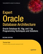
This is a term used with table segments stored in the database. If you envision a table, for example, as a flat structure or as a series of blocks laid one after the other in a line from left to right, the high-water mark (HWM) would be the rightmost block that ever contained data, as illustrated in Figure 10-1.

Figure 10-1. Depiction of an HWM

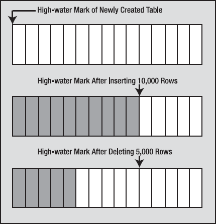
Figure 10-1 shows that the HWM starts at the first block of a newly created table. As data is placed into the table over time and more blocks get used, the HWM rises. If we delete some (or even all) of the rows in the table, we might have many blocks that no longer contain data, but they are still under the HWM, and they will remain under the HWM until the object is rebuilt, truncated, or shrunk (shrinking of a segment is a new Oracle 10g feature that is supported only if the segment is in an ASSM tablespace).

The HWM is relevant since Oracle will scan all blocks under the HWM, even when they contain no data, during a full scan. This will impact the performance of a full scan—especially if most of the blocks under the HWM are empty. To see this, just create a table with 1,000,000 rows (or create any table with a large number of rows), and then execute a SELECT COUNT(*) from this table. Now, DELETE every row in it and you will find that the SELECT COUNT(*) takes just as long (or longer, if you need to clean out the block! Refer to the "Block Cleanout" section of Chapter 9 "Redo and Undo" to count 0 rows as it did to count 1,000,000. This is because Oracle is busy reading all of the blocks below the HWM to see if they contain data. You should compare this to what happens if you used TRUNCATE on the table instead of deleting each individual row. TRUNCATE will reset the HWM of a table back to zero and will truncate the associated indexes on the table as well. If you plan on deleting every row in a table, TRUNCATE—if it can be used—would be the method of choice for this reason.

In an MSSM tablespace, segments have a definite HWM. In an ASSM tablespace, however, there is an HWM and a low HWM. In MSSM, when the HWM is advanced (e.g., as rows are inserted), all of the blocks are formatted and valid, and Oracle can read them safely. With ASSM, however, when the HWM is advanced Oracle doesn't format all of the blocks immediately—they are only formatted and made safe to read upon their first actual use. The first actual use will be when the database decides to insert a record into a given block. Under ASSM, the data is inserted in any of the blocks between the low high water mark and the high water mark, so many of the blocks in this area might not be formatted. So, when full scanning a segment, we have to know if the blocks to be read are safe or unformatted (meaning they contain nothing of interest and we do not process them). To make it so that not every block in the table needs go through this safe/not safe check, Oracle maintains a low HWM and a HWM. Oracle will full scan the table up to the HWM—and for all of the blocks below the low HWM, it will just read and process them. For blocks between the low HWM and the HWM (see Figure 10-2), it must be more careful and refer to the ASSM bitmap information used to manage these blocks in order to see which of them it should read and which it should just ignore.

Figure 10-2. Depiction of a low HWM

ops$tkyte%ORA11GR2> create table t ( x int, y char(50) ) tablespace mssm;
Table created.

begin
    for i in 1 .. 100000
    loop
        insert into t values ( i, 'x' );
    end loop;
    commit;
end;
/
exit;

Snapshot       Snap Id     Snap Time      Sessions Curs/Sess Comment
~~~~~~~~    ---------- ------------------ -------- --------- ------------------
Begin Snap:        364 17-Mar-10 11:58:24       26       1.7
  End Snap:        365 17-Mar-10 11:59:01       24       1.8
   Elapsed:       0.62 (mins) Av Act Sess:       4.9
   DB time:       3.04 (mins)      DB CPU:       1.18 (mins)

Top 5 Timed Events                                                    Avg %Total
~~~~~~~~~~~~~~~~~~                                                   wait   Call
Event                                            Waits    Time (s)   (ms)   Time
----------------------------------------- ------------ ----------- ------ ------
buffer busy waits                              199,708         107      1   53.5
CPU time                                                        70          35.0
db file async I/O submit                            44          11    252    5.5
log file parallel write                          1,130           9      8    4.5
control file parallel write                         56           1     16     .4
          -------------------------------------------------------------

ops$tkyte@ORA11GR2> create table t ( x int, y char(50) )
   2  storage ( freelists 5 ) tablespace MSSM;
Table created.

ops$tkyteORA11GR2> alter table t storage ( FREELISTS 5 );
Table altered.

Snapshot       Snap Id     Snap Time      Sessions Curs/Sess Comment
~~~~~~~~    ---------- ------------------ -------- --------- ------------------
Begin Snap:        367 17-Mar-10 12:26:50       24       1.3
  End Snap:        368 17-Mar-10 12:27:09       22       1.5
   Elapsed:       0.32 (mins) Av Act Sess:       4.3
   DB time:       1.37 (mins)      DB CPU:       0.98 (mins)

Top 5 Timed Events                                                    Avg %Total
~~~~~~~~~~~~~~~~~~                                                   wait   Call
Event                                            Waits    Time (s)   (ms)   Time
----------------------------------------- ------------ ----------- ------ ------
CPU time                                                        59          59.9
db file async I/O submit                            28          15    536   15.3
log file parallel write                            752          10     13    9.8
buffer busy waits                               17,929           5      0    5.4
cursor: pin S                                      252           3     11    2.9

ops$tkyte@ORA11GR2> create tablespace assm
  2  datafile size 1m autoextend on next 1m
  3  segment space management auto;
Tablespace created.

ops$tkyte@ORA11GR2> create table t ( x int, y char(50) ) tablespace ASSM;
Table created.

Snapshot       Snap Id     Snap Time      Sessions Curs/Sess Comment
~~~~~~~~    ---------- ------------------ -------- --------- ------------------
Begin Snap:        369 17-Mar-10 12:31:05       22       1.5
  End Snap:        370 17-Mar-10 12:31:25       24       1.3
   Elapsed:       0.33 (mins) Av Act Sess:       4.6
   DB time:       1.54 (mins)      DB CPU:       1.08 (mins)

Top 5 Timed Events                                                    Avg %Total
~~~~~~~~~~~~~~~~~~                                                   wait   Call
Event                                            Waits    Time (s)   (ms)   Time
----------------------------------------- ------------ ----------- ------ ------
CPU time                                                        65          58.2
db file async I/O submit                            25          17    661   14.9
log file parallel write                            674          11     16    9.8
log file switch (checkpoint incomplete)             13           4    334    3.9
buffer busy waits                                7,642           4      0    3.4

PCTFREE and PCTUSED

In general, the PCTFREE parameter tells Oracle how much space should be reserved on a block for future updates. By default, this is 10 percent. If there is a higher percentage of free space than the value specified in PCTFREE, then the block is considered to be free. PCTUSED tells Oracle the percentage of free space that needs to be present on a block that is not currently free in order for it to become free again. The default value is 40 percent.

As noted earlier, when used with a table (but not an IOT, as we'll see), PCTFREE tells Oracle how much space should be reserved on a block for future updates. This means if we use an 8KB block size, as soon as the addition of a new row onto a block causes the free space on the block to drop below about 800 bytes, Oracle will use another block from the FREELIST instead of the existing block. This 10 percent of the data space on the block is set aside for updates to the rows on that block.

Note

PCTFREE and PCTUSED are implemented differently for different table types. Some table types employ both, whereas others only use PCTFREE, and even then only when the object is created. IOTs use PCTFREE upon creation to set aside space in the table for future updates, but do not use PCTFREE to decide when to stop inserting rows into a given block, for example.

The exact effect of these two parameters varies depending on whether you are using ASSM or MSSM tablespaces. When you are using MSSM, these parameter settings control when the block will be put on and taken off the FREELIST. If you are using the default values for PCTFREE (10) and PCTUSED (40), then a block will remain on the FREELIST until it is 90 percent full (10 percent free space). Once it hits 90 percent, it will be taken off the FREELIST and remain off the FREELIST until the free space on the block exceeds 60 percent of the block.

When you are using ASSM, PCTFREE still limits if a new row may be inserted into a block, but it does not control whether a block is on a FREELIST or not, as ASSM does not use FREELISTs at all. In ASSM, PCTUSED is simply ignored.

There are three settings for PCTFREE: too high, too low, and just about right. If you set PCTFREE for blocks too high, you will waste space. If you set PCTFREE to 50 percent and you never update the data, you have just wasted 50 percent of every block. On another table, however, 50 percent may be very reasonable. If the rows start out small and tend to double in size, setting PCTFREE too small will cause row migration as you update the rows.

Row Migration

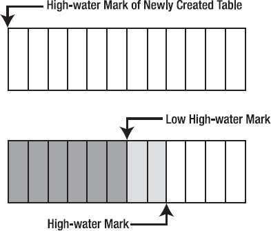
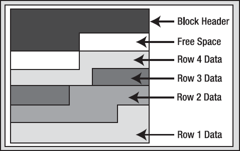
What is row migration? Row migration is when a row is forced to leave the block it was created on because it grew too large to fit on that block with the rest of the rows. To illustrate row migration, we start with a block that looks like Figure 10-3.

Figure 10-3. Data block before update

Approximately one-seventh of the block is free space. However, we would like to more than double the amount of space used by row 4 via an UPDATE (it currently consumes one-seventh of the block). In this case, even if Oracle coalesced the space on the block as shown in Figure 10-4, there is still insufficient room to double the size of row 4, because the size of the free space is less than the current size of row 4.

Figure 10-4. Data block as it would appear after coalescing free space

If the row fit into the coalesced space, it would have happened. This time, however, Oracle will not perform this coalescing and the block will remain as it is. Since row 4 would have to span more than one block if it stayed on this block, Oracle will move, or migrate, the row. However, Oracle cannot just move the row; it must leave behind a forwarding address. There may be indexes that physically point to this address for row 4. A simple update will not modify the indexes as well.

Note

There is a special case with partitioned tables that a rowid, the address of a row, will change. We will look at this case in Chapter 13 "Partitioning." Additionally, other administrative operations such as FLASHBACK TABLE and ALTER TABLE SHRINK may change rowids assigned to rows as well.

Therefore, when Oracle migrates the row, it will leave behind a pointer to where the row really is. After the update, the blocks might look as shown in Figure 10-5.

Figure 10-5. Migrated row depiction

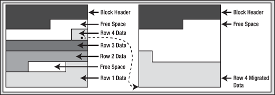
So, a migrated row is a row that had to move from the block it was inserted into onto some other block. Why is this an issue? Your application will never know; the SQL you use is no different. It only matters for performance reasons. If you go to read this row via an index, the index will point to the original block. That block will point to the new block. Instead of doing the two or so I/Os to read the index plus one I/O to read the table, you'll need to do yet one more I/O to get to the actual row data. In isolation, this is no big deal—you won't even notice it. However, when you have a sizable percentage of your rows in this state, with many users accessing them, you'll begin to notice this side effect. Access to this data will start to slow down (additional I/Os and the associated latching that goes with the I/O add to the access time), your buffer cache efficiency goes down (you need to buffer two blocks instead of just the one you would if the rows were not migrated), and your table grows in size and complexity. For these reasons, you generally do not want migrated rows (but do not lose sleep if a couple hundred/thousand rows in a table of thousands or more rows are migrated!).

It is interesting to note what Oracle will do if the row that was migrated from the block on the left to the block on the right in Figure 10-5 has to migrate again at some future point in time. This would be due to other rows being added to the block it was migrated to and then updating this row to make it even larger. Oracle will actually migrate the row back to the original block and, if there is sufficient space, leave it there (the row might become unmigrated). If there isn't sufficient space, Oracle will migrate the row to another block altogether and change the forwarding address on the original block. As such, row migrations will always involve one level of indirection.

So, now we are back to PCTFREE and what it is used for: it is the setting that will help you to minimize row migration and row chaining (discussed later) when set properly.

Setting PCTFREE and PCTUSED Values

Setting PCTFREE and PCTUSED is an important—and greatly overlooked—topic. In summary, PCTUSED and PCTFREE are both crucial when using MSSM; with ASSM, only PCTFREE is. On the one hand, you need to use them to avoid too many rows from migrating. On the other hand, you use them to avoid wasting too much space. You need to look at your objects and describe how they will be used, and then you can come up with a logical plan for setting these values. Rules of thumb may very well fail you on these settings; they really need to be set based on usage. You might consider the following (keeping in mind that "high" and "low" are relative terms, and that when using ASSM, only PCTFREE applies):

• High PCTFREE, low PCTUSED: This setting is for when you insert lots of data that will be updated, and the updates will increase the size of the rows frequently. This setting reserves a lot of space on the block after inserts (high PCTFREE) and makes it so that the block must almost be empty before getting back onto the FREELIST (low PCTUSED).

• Low PCTFREE, high PCTUSED: This setting is for if you tend to only ever INSERT or DELETE from the table, or if you do UPDATE, the UPDATE tends to shrink the row in size.

A heap organized table is probably used 99 percent (or more) of the time in applications. A heap organized table is the type of table you get by default when you issue the CREATE TABLE statement. If you want any other type of table structure, you need to specify that in the CREATE statement itself.

A heap is a classic data structure studied in computer science. It is basically a big area of space, disk, or memory (disk in the case of a database table, of course) that is managed in an apparently random fashion. Data will be placed where it fits best, rather than in any specific sort of order. Many people expect data to come back out of a table in the same order it was put into it, but with a heap, this is definitely not assured. In fact, rather the opposite is guaranteed: the rows will come out in a wholly unpredictable order. This is quite easy to demonstrate.

In this example, I will set up a table such that in my database I can fit one full row per block (I am using an 8KB block size). You do not need to have the case where you only have one row per block— I am just taking advantage of this to demonstrate a predictable sequence of events. The following sort of behavior (that rows have no order) will be observed on tables of all sizes, in databases with any block size:

ops$tkyte%ORA11GR2> create table t
  2  ( a int,
  3    b varchar2(4000) default rpad('*',4000,'*'),
  4    c varchar2(3000) default rpad('*',3000,'*')
  5  )
  6  /
Table created.

ops$tkyte%ORA11GR2> insert into t (a) values ( 1);
1 row created.

ops$tkyte%ORA11GR2> insert into t (a) values ( 2);
1 row created.

ops$tkyte%ORA11GR2> insert into t (a) values ( 3);
1 row created.

ops$tkyte%ORA11GR2> delete from t where a = 2 ;
1 row deleted.

ops$tkyte%ORA11GR2> insert into t (a) values ( 4);
1 row created.

ops$tkyte%ORA11GR2> select a from t;

         A
----------
         1
         4
         3

Adjust columns B and C to be appropriate for your block size if you would like to reproduce this. For example, if you have a 2KB block size, you do not need column C, and column B should be a VARCHAR2(1500) with a default of 1,500 asterisks. Since data is managed in a heap in a table like this, as space becomes available, it will be reused.

A full scan of the table will retrieve the data as it hits it, not in the order of insertion. This is a key concept to understand about database tables: in general, they are inherently unordered collections of data. You should also note that I do not need to use a DELETE in order to observe this effect; I could achieve the same results using only INSERTs. If I insert a small row, followed by a very large row that will not fit on the block with the small row, and then a small row again, I may very well observe that the rows come out by default in the order "small row, small row, large row." They will not be retrieved in the order of insertion—Oracle will place the data where it fits, not in any order by date or transaction.

If your query needs to retrieve data in order of insertion, you must add a column to the table that you can use to order the data when retrieving it. This column could be a number column, for example, maintained with an increasing sequence (using the Oracle SEQUENCE object). You could then approximate the insertion order using a SELECT that did an ORDER BY on this column. It will be an approximation because the row with sequence number 55 may very well have committed before the row with sequence 54, therefore it was officially first in the database.

You should think of a heap organized table as a big unordered collection of rows. These rows will come out in a seemingly random order, and depending on other options being used (parallel query, different optimizer modes, and so on), they may come out in a different order with the same query. Do not ever count on the order of rows from a query unless you have an ORDER BY statement on your query!

That aside, what is important to know about heap tables? Well, the CREATE TABLE syntax spans some 72 pages in the SQL Reference Manual provided by Oracle, so there are lots of options that go along with them. There are so many options that getting a hold on all of them is pretty difficult. The wire diagrams (or train track diagrams) alone take 18 pages to cover. One trick I use to see most of the options available to me in the CREATE TABLE statement for a given table is to create the table as simply as possible, for example:

ops$tkyte@ORA11GR2> create table t
  2  ( x int primary key,
  3    y date,
  4    z clob
  5  )
  6  /
Table created.

Then, using the standard supplied package DBMS_METADATA, I query the definition of it and see the verbose syntax:

ops$tkyte%ORA11GR2> select dbms_metadata.get_ddl( 'TABLE', 'T' ) from dual;

DBMS_METADATA.GET_DDL('TABLE','T')
------------------------------------------------------------------------------

  CREATE TABLE "OPS$TKYTE"."T"
   (    "X" NUMBER(*,0),
        "Y" DATE,
        "Z" CLOB,
         PRIMARY KEY ("X")
  USING INDEX PCTFREE 10 INITRANS 2 MAXTRANS 255 NOCOMPRESS LOGGING
  TABLESPACE "USERS"  ENABLE
   ) SEGMENT CREATION DEFERRED
  PCTFREE 10 PCTUSED 40 INITRANS 1 MAXTRANS 255 NOCOMPRESS LOGGING
  TABLESPACE "USERS"
 LOB ("Z") STORE AS BASICFILE (
  TABLESPACE "USERS" ENABLE STORAGE IN ROW CHUNK 8192 RETENTION
  NOCACHE LOGGING )

The nice thing about this trick is that it shows many of the options for my CREATE TABLE statement. I just have to pick data types and such; Oracle will produce the verbose version for me. I can now customize this verbose version, perhaps changing the ENABLE STORAGE IN ROW to DISABLE STORAGE IN ROW, which would disable the storage of the LOB data in the row with the structured data, causing it to be stored in another segment. I use this trick myself all of the time to avoid having to decipher the huge wire diagrams. I also use this technique to learn what options are available to me on the CREATE TABLE statement under different circumstances.

Now that you know how to see most of the options available to you on a given CREATE TABLE statement, which are the important ones you need to be aware of for heap tables? In my opinion, there are three with ASSM and five with MSSM:

These are the parameters you want to pay particularly close attention to. With the introduction of locally managed tablespaces, which are highly recommended, I find that the rest of the storage parameters (such as PCTINCREASE, NEXT, and so on) are simply not relevant anymore.

Index organized tables (IOTs) are quite simply tables stored in an index structure. Whereas a table stored in a heap is unorganized (i.e., data goes wherever there is available space), data in an IOT is stored and sorted by primary key. IOTs behave just like "regular" tables do as far as your application is concerned; you use SQL to access them as normal. They are especially useful for information retrieval, spatial, and OLAP applications.

What is the point of an IOT? You might ask the converse, actually: what is the point of a heap organized table? Since all tables in a relational database are supposed to have a primary key anyway, isn't a heap organized table just a waste of space? We have to make room for both the table and the index on the primary key of the table when using a heap organized table. With an IOT, the space overhead of the primary key index is removed, as the index is the data, and the data is the index. The fact is that an index is a complex data structure that requires a lot of work to manage and maintain, and the maintenance requirements increase as the width of the row to store increases. A heap, on the other hand, is trivial to manage by comparison. There are efficiencies in a heap organized table over an IOT. That said, IOTs have some definite advantages over their heap counterparts. For example, I once built an inverted list index on some textual data (this predated the introduction of interMedia and related technologies). I had a table full of documents, and I would parse the documents and find words within them. My table looked like this:

create table keywords
( word  varchar2(50),
  position   int,
  doc_id int,
  primary key(word,position,doc_id)
);

Here I had a table that consisted solely of columns of the primary key. I had over 100 percent overhead; the size of my table and primary key index were comparable (actually, the primary key index was larger since it physically stored the rowid of the row it pointed to, whereas a rowid is not stored in the table—it is inferred). I only used this table with a WHERE clause on the WORD or WORD and POSITION columns. That is, I never used the table—I used only the index on the table. The table itself was no more than overhead. I wanted to find all documents containing a given word (or near another word, and so on). The KEYWORDS heap table was useless, and it just slowed down the application during maintenance of the KEYWORDS table and doubled the storage requirements. This is a perfect application for an IOT.

Another implementation that begs for an IOT is a code lookup table. Here you might have ZIP_CODE to STATE lookup, for example. You can now do away with the heap table and just use an IOT itself. Anytime you have a table that you access via its primary key exclusively, it is a possible candidate for an IOT.

When you want to enforce co-location of data or you want data to be physically stored in a specific order, the IOT is the structure for you. For users of Sybase and SQL Server, this is where you would have used a clustered index, but IOTs go one better. A clustered index in those databases may have up to a 110 percent overhead (similar to the previous KEYWORDS table example). Here, we have a 0 percent overhead since the data is stored only once. A classic example of when you might want this physically co-located data would be in a parent/child relationship. Let's say the EMP table had a child table containing addresses. You might have a home address entered into the system when the employee is initially sent an offer letter for a job. Later, he adds his work address. Over time, he moves and changes the home address to a previous address and adds a new home address. Then he has a school address he added when he went back for a degree, and so on. That is, the employee has three or four (or more) detail records, but these details arrive randomly over time. In a normal heap based table, they just go anywhere. The odds that two or more of the address records would be on the same database block in the heap table are very near zero. However, when you query an employee's information, you always pull the address detail records as well. The rows that arrive over time are always retrieved together. To make the retrieval more efficient, you can use an IOT for the child table to put all of the records for a given employee near each other upon insertion, so when you retrieve them over and over again, you do less work.

An example will easily show the effects of using an IOT to physically co-locate the child table information. Let's create and populate an EMP table:

ops$tkyte%ORA11GR2> create table emp
  2  as
  3  select object_id   empno,
  4         object_name ename,
  5         created     hiredate,
  6         owner       job
  7    from all_objects
  8  /

Table created.

ops$tkyte%ORA11GR2> alter table emp add constraint emp_pk primary key(empno)
  2  /

Table altered.

ops$tkyte%ORA11GR2> begin
  2     dbms_stats.gather_table_stats( user, 'EMP', cascade=>true );
  3  end;
  4  /

PL/SQL procedure successfully completed.

Next, we'll implement the child table two times, once as a conventional heap table and again as an IOT:

ops$tkyte%ORA11GR2> create table heap_addresses
  2  ( empno     references emp(empno) on delete cascade,
  3    addr_type varchar2(10),
  4    street    varchar2(20),
  5    city      varchar2(20),
  6    state     varchar2(2),
  7    zip       number,

8    primary key (empno,addr_type)
  9  )
 10  /

Table created.

ops$tkyte%ORA11GR2> create table iot_addresses
  2  ( empno     references emp(empno) on delete cascade,
  3    addr_type varchar2(10),
  4    street    varchar2(20),
  5    city      varchar2(20),
  6    state     varchar2(2),
  7    zip       number,
  8    primary key (empno,addr_type)
  9  )
 10  ORGANIZATION INDEX
 11  /

Table created.

I populated these tables by inserting into them a work address for each employee, then a home address, then a previous address, and finally a school address. A heap table would tend to place the data at the end of the table; as the data arrives, the heap table would simply add it to the end, due to the fact that the data is just arriving and no data is being deleted. Over time, if addresses are deleted, the inserts would become more random throughout the table. Suffice it to say, the chance an employee's work address would be on the same block as his home address in the heap table is near zero. For the IOT, however, since the key is on EMPNO, ADDR_TYPE, we'll be pretty sure that all of the addresses for a given EMPNO are located on one or maybe two index blocks together. The inserts used to populate this data were:

ops$tkyte%ORA11GR2> insert into heap_addresses
  2  select empno, 'WORK', '123 main street', 'Washington', 'DC', 20123
  3    from emp;
72075 rows created.

ops$tkyte%ORA11GR2> insert into iot_addresses
  2  select empno, 'WORK', '123 main street', 'Washington', 'DC', 20123
  3    from emp;
72075 rows created.

I did that three more times, changing WORK to HOME, PREV, and SCHOOL in turn. Then I gathered statistics:

ops$tkyte%ORA11GR2> exec dbms_stats.gather_table_stats( user, 'HEAP_ADDRESSES' );
PL/SQL procedure successfully completed.

ops$tkyte%ORA11GR2> exec dbms_stats.gather_table_stats( user, 'IOT_ADDRESSES' );
PL/SQL procedure successfully completed.

Now we are ready to see what measurable difference we could expect to see. Using AUTOTRACE, we'll get a feeling for the change:

ops$tkyte%ORA11GR2> set autotrace traceonly
ops$tkyte%ORA11GR2> select *
  2    from emp, heap_addresses
  3   where emp.empno = heap_addresses.empno
  4     and emp.empno = 42;


Execution Plan
----------------------------------------------------------
Plan hash value: 4163174643

-----------------------------------------------------------------------
| Id  | Operation                    | Name           | Rows  | Bytes |
-----------------------------------------------------------------------
|   0 | SELECT STATEMENT             |                |     4 |   356 |
|   1 |  NESTED LOOPS                |                |     4 |   356 |
|   2 |   TABLE ACCESS BY INDEX ROWID| EMP            |     1 |    43 |
|*  3 |    INDEX UNIQUE SCAN         | EMP_PK         |     1 |       |
|   4 |   TABLE ACCESS BY INDEX ROWID| HEAP_ADDRESSES |     4 |   184 |
|*  5 |    INDEX RANGE SCAN          | SYS_C0019080   |     4 |       |
-----------------------------------------------------------------------

Predicate Information (identified by operation id):
---------------------------------------------------

   3 - access("EMP"."EMPNO"=42)
   5 - access("HEAP_ADDRESSES"."EMPNO"=42)


Statistics
----------------------------------------------------------
          0  recursive calls
          0  db block gets
         11  consistent gets
          0  physical reads
          0  redo size
       1153  bytes sent via SQL*Net to client
        419  bytes received via SQL*Net from client
          2  SQL*Net roundtrips to/from client
          0  sorts (memory)
          0  sorts (disk)
          4  rows processed

That is a pretty common plan: go to the EMP table by primary key; get the row; then using that EMPNO, go to the address table; and using the index, pick up the child records. We did 11 I/Os to retrieve this data. Now running the same query, but using the IOT for the addresses

ops$tkyte%ORA11GR2> select *
  2    from emp, iot_addresses
  3   where emp.empno = iot_addresses.empno

4     and emp.empno = 42;


Execution Plan
----------------------------------------------------------
Plan hash value: 1490857195

--------------------------------------------------------------------------
| Id  | Operation                    | Name              | Rows  | Bytes |
--------------------------------------------------------------------------
|   0 | SELECT STATEMENT             |                   |     4 |   356 |
|   1 |  NESTED LOOPS                |                   |     4 |   356 |
|   2 |   TABLE ACCESS BY INDEX ROWID| EMP               |     1 |    43 |
|*  3 |    INDEX UNIQUE SCAN         | EMP_PK            |     1 |       |
|*  4 |   INDEX RANGE SCAN           | SYS_IOT_TOP_93124 |     4 |   184 |
--------------------------------------------------------------------------

Predicate Information (identified by operation id):
---------------------------------------------------

   3 - access("EMP"."EMPNO"=42)
   4 - access("IOT_ADDRESSES"."EMPNO"=42)


Statistics
----------------------------------------------------------
          0  recursive calls
          0  db block gets
          7  consistent gets
          0  physical reads
          0  redo size
       1153  bytes sent via SQL*Net to client
        419  bytes received via SQL*Net from client
          2  SQL*Net roundtrips to/from client
          0  sorts (memory)
          0  sorts (disk)
          4  rows processed

we did four fewer I/Os (the four should have been guessable); we skipped four TABLE ACCESS (BY INDEX ROWID) steps. The more child records we have, the more I/Os we would anticipate skipping.

So, what is four I/Os? Well, in this case it was over one-third of the I/O performed for the query, and if we execute this query repeatedly, it would add up. Each I/O and each consistent get requires an access to the buffer cache, and while it is true that reading data out of the buffer cache is faster than disk, it is also true that the buffer cache gets are not free and not totally cheap. Each will require many latches of the buffer cache, and latches are serialization devices that will inhibit our ability to scale. We can measure both the I/O reduction as well as latching reduction by running a PL/SQL block such as this:

ops$tkyte%ORA11GR2> begin
  2      for x in ( select empno from emp )
  3      loop
  4          for y in ( select emp.ename, a.street, a.city, a.state, a.zip
  5                       from emp, heap_addresses a
  6                      where emp.empno = a.empno

7                        and emp.empno = x.empno )
  8          loop
  9              null;
 10          end loop;
 11       end loop;
 12  end;
 13  /

PL/SQL procedure successfully completed.

Here, we are just emulating a busy period and running the query some 45,000 times, once for each EMPNO. If we run that for the HEAP_ADRESSES and IOT_ADDRESSES tables, TKPROF shows us the following:

SELECT EMP.ENAME, A.STREET, A.CITY, A.STATE, A.ZIP
FROM  EMP, HEAP_ADDRESSES A WHERE EMP.EMPNO = A.EMPNO AND EMP.EMPNO = :B1

call     count       cpu    elapsed       disk      query    current        rows
------- ------  -------- ---------- ---------- ---------- ----------  ----------
Parse        1      0.00       0.00          0          0          0           0
Execute  72073     11.53      11.79          0          0          0           0
Fetch    72073      6.55       6.58       3641     722160          0      288292
------- ------  -------- ---------- ---------- ---------- ----------  ----------
total   144147     18.09      18.38       3641     722160          0      288292

Misses in library cache during parse: 0
Optimizer mode: ALL_ROWS
Parsing user id: 286     (recursive depth: 1)

Rows     Row Source Operation
-------  ---------------------------------------------------
      4  NESTED LOOPS  (cr=10 pr=0 pw=0 time=60 us cost=8 size=280 card=4)
      1   TABLE ACCESS BY INDEX ROWID EMP (cr=3 pr=0 pw=0 time=0 us cost=2 siz...)
      1    INDEX UNIQUE SCAN EMP_PK (cr=2 pr=0 pw=0 time=0 us cost=1 size=0 ...)
      4   TABLE ACCESS BY INDEX ROWID HEAP_ADDRESSES (cr=7 pr=0 pw=0 time=54 us...)
      4    INDEX RANGE SCAN SYS_C0019080 (cr=3 pr=0 pw=0 time=3 us cost=2 size=...)
********************************************************************************
SELECT EMP.ENAME, A.STREET, A.CITY, A.STATE, A.ZIP
FROM
 EMP, IOT_ADDRESSES A WHERE EMP.EMPNO = A.EMPNO AND EMP.EMPNO = :B1

call     count       cpu    elapsed       disk      query    current        rows
------- ------  -------- ---------- ---------- ---------- ----------  ----------
Parse        1      0.00       0.00          0          0          0           0
Execute  72073     11.61      11.74          0          0          0           0
Fetch    72073      4.70       4.78       4863     437132          0      288292
------- ------  -------- ---------- ---------- ---------- ----------  ----------
total   144147     16.32      16.52       4863     437132          0      288292

Misses in library cache during parse: 0
Optimizer mode: ALL_ROWS
Parsing user id: 286     (recursive depth: 1)

Rows     Row Source Operation
-------  ---------------------------------------------------
      4  NESTED LOOPS  (cr=7 pr=3 pw=0 time=9 us cost=4 size=280 card=4)
      1   TABLE ACCESS BY INDEX ROWID EMP (cr=3 pr=0 pw=0 time=0 us cost=2 size=30...)
      1    INDEX UNIQUE SCAN EMP_PK (cr=2 pr=0 pw=0 time=0 us cost=1 size=0 ...)
      4   INDEX RANGE SCAN SYS_IOT_TOP_93124 (cr=4 pr=3 pw=0 time=3 us cost=2 ...)

Both queries fetched exactly the same number of rows, but the HEAP table performed considerably more logical I/O. As the degree of concurrency on the system goes up, we would likewise expect the CPU used by the HEAP table to go up more rapidly as well, while the query possibly waits for latches into the buffer cache. Using runstats (a utility of my own design; refer to the introductory section "Setting Up Your Environment for This Book" for details), we can measure the difference in latching. On my system, I observed the following

STAT...consistent gets             723,073     438,048    −285,025
STAT...consistent gets from ca     723,073     438,048    −285,025
STAT...no work - consistent re     362,683      77,651    −285,032
STAT...session logical reads       723,131     438,086    −285,045
STAT...consistent gets from ca     359,225      72,982    −286,243
STAT...table fetch by rowid        360,385      72,085    −288,300
STAT...buffer is not pinned co     648,695     288,324    −360,371
LATCH.cache buffers chains       1,090,022     523,161    −566,861
STAT...physical read total byt  30,703,616  40,747,008  10,043,392
STAT...physical read bytes      30,703,616  40,747,008  10,043,392
STAT...cell physical IO interc  30,703,616  40,747,008  10,043,392

Run1 latches total versus runs -- difference and pct
Run1        Run2        Diff       Pct
1,204,593     624,834    −579,759    192.79%

where Run1 was the HEAP_ADDRESSES table and Run2 was the IOT_ADDRESSES table. As you can see, there was a dramatic and repeatable decrease in the latching taking place, mostly due to the cache buffers chains latch (the one that protects the buffer cache). The IOT in this case would provide the following benefits:

The same would be true if you frequently use BETWEEN queries on a primary or unique key. Having the data stored physically sorted will increase the performance of those queries as well. For example, I maintain a table of stock quotes in my database. Every day, for hundreds of stocks, I gather together the stock ticker, date, closing price, days high, days low, volume, and other related information. The table looks like this:

ops$tkyte@ORA11GR2> create table stocks
  2  ( ticker      varchar2(10),
  3    day         date,

4    value       number,
  5    change      number,
  6    high        number,
  7    low         number,
  8    vol         number,
  9    primary key(ticker,day)
 10  )
 11  organization index
 12  /
Table created.

I frequently look at one stock at a time for some range of days (e.g., computing a moving average). If I were to use a heap organized table, the probability of two rows for the stock ticker ORCL existing on the same database block are almost zero. This is because every night, I insert the records for the day for all of the stocks. This fills up at least one database block (actually, many of them). Therefore, every day I add a new ORCL record, but it is on a block different from every other ORCL record already in the table. If I query as follows

Select * from stocks
 where ticker = 'ORCL'
   and day between sysdate-100 and sysdate;

Oracle would read the index and then perform table access by rowid to get the rest of the row data. Each of the 100 rows I retrieve would be on a different database block due to the way I load the table—each would probably be a physical I/O. Now consider that I have this same data in an IOT. That same query only needs to read the relevant index blocks, and it already has all of the data. Not only is the table access removed, but all of the rows for ORCL in a given range of dates are physically stored near each other as well. Less logical I/O and less physical I/O is incurred.

Now you understand when you might want to use IOTs and how to use them. What you need to understand next is what the options are with these tables. What are the caveats? The options are very similar to the options for a heap organized table. Once again, we'll use DBMS_METADATA to show us the details. Let's start with the three basic variations of the IOT:

ops$tkyte%ORA11GR2> create table t1
  2  (  x int primary key,
  3     y varchar2(25),
  4     z date
  5  )
  6  organization index;
Table created.

ops$tkyte%ORA11GR2> create table t2
  2  (  x int primary key,
  3     y varchar2(25),
  4     z date
  5  )
  6  organization index
  7  OVERFLOW;
Table created.

ops$tkyte%ORA11GR2> create table t3
  2  (  x int primary key,
  3     y varchar2(25),

4     z date
  5  )
  6  organization index
  7  overflow INCLUDING y;

Table created.

We'll get into what OVERFLOW and INCLUDING do for us, but first let's look at the detailed SQL required for the first table:

ops$tkyte%ORA11GR2> select dbms_metadata.get_ddl( 'TABLE', 'T1' ) from dual;

DBMS_METADATA.GET_DDL('TABLE','T1')
-------------------------------------------------------------------------------

  CREATE TABLE "OPS$TKYTE"."T1"
   (    "X" NUMBER(*,0),
        "Y" VARCHAR2(25),
        "Z" DATE,
         PRIMARY KEY ("X") ENABLE
   ) ORGANIZATION INDEX NOCOMPRESS PCTFREE 10 INITRANS 2 MAXTRANS 255 LOGGING
  STORAGE(INITIAL 65536 NEXT 1048576 MINEXTENTS 1 MAXEXTENTS 2147483645
  PCTINCREASE 0 FREELISTS 1 FREELIST GROUPS 1 BUFFER_POOL DEFAULT FLASH_CACHE
DEFAULT CELL_FLASH_CACHE DEFAULT)
  TABLESPACE "USERS"
 PCTTHRESHOLD 50

This table introduces a new option, PCTTHRESHOLD, which we'll look at in a moment. You might have noticed that something is missing from the preceding CREATE TABLE syntax: there is no PCTUSED clause, but there is a PCTFREE. This is because an index is a complex data structure that isn't randomly organized like a heap, so data must go where it belongs. Unlike a heap, where blocks are sometimes available for inserts, blocks are always available for new entries in an index. If the data belongs on a given block because of its values, it will go there regardless of how full or empty the block is. Additionally, PCTFREE is used only when the object is created and populated with data in an index structure. It is not used like it is in the heap organized table. PCTFREE will reserve space on a newly created index, but not for subsequent operations on it, for much the same reason as PCTUSED is not used at all. The same considerations for FREELISTs we had on heap organized tables apply in whole to IOTs.

First, let's look at the NOCOMPRESS option. This option is different in implementation from the table compression discussed above. It works for any operation on the index organized table (as opposed to the table compression which may or may not be in effect for conventional path operations). Using NOCOMPRESS, it tells Oracle to store each and every value in an index entry (i.e., do not compress). If the primary key of the object were on columns A, B, and C, every occurrence of A, B, and C would physically be stored. The converse to NOCOMPRESS is COMPRESS N, where N is an integer that represents the number of columns to compress. This removes repeating values and factors them out at the block level, so that the values of A and perhaps B that repeat over and over are no longer physically stored. Consider, for example, a table created like this:

ops$tkyte%ORA11GR2> create table iot
  2  ( owner, object_type, object_name,
  3    primary key(owner,object_type,object_name)
  4  )
  5  organization index
  6  NOCOMPRESS

7  as
  8  select distinct owner, object_type, object_name from all_objects
/
Table created.

It you think about it, the value of OWNER is repeated many hundreds of times. Each schema (OWNER) tends to own lots of objects. Even the value pair of OWNER,OBJECT_TYPE repeats many times, so a given schema will have dozens of tables, dozens of packages, and so on. Only all three columns together do not repeat. We can have Oracle suppress these repeating values. Instead of having an index block with values shown in Table 10-1, we could use COMPRESS 2 (factor out the leading two columns) and have a block with the values shown in Table 10-2.

That is, the values SYS and TABLE appear once, and then the third column is stored. In this fashion, we can get many more entries per index block than we could otherwise. This does not decrease concurrency—we are still operating at the row level in all cases—or functionality at all. It may use slightly more CPU horsepower, as Oracle has to do more work to put together the keys again. On the other hand, it may significantly reduce I/O and allow more data to be cached in the buffer cache, since we get more data per block. That is a pretty good tradeoff.

Let's demonstrate the savings by doing a quick test of the preceding CREATE TABLE as SELECT with NOCOMPRESS, COMPRESS 1, and COMPRESS 2. We'll start by creating our IOT without compression:

ops$tkyte%ORA11GR2> create table iot
  2  ( owner, object_type, object_name,
  3    constraint iot_pk primary key(owner,object_type,object_name)
  4  )
  5  organization index
  6  NOCOMPRESS
  7  as
  8  select distinct owner, object_type, object_name

9    from all_objects
 10  /
Table created.

Now we can measure the space used. We'll use the ANALYZE INDEX VALIDATE STRUCTURE command for this. This command populates a dynamic performance view named INDEX_STATS, which will contain only one row at most with the information from the last execution of that ANALYZE command:

ops$tkyte%ORA11GR2> analyze index iot_pk validate structure;
Index analyzed.

ops$tkyte%ORA11GR2> select lf_blks, br_blks, used_space,
  2         opt_cmpr_count, opt_cmpr_pctsave
  3    from index_stats;

   LF_BLKS    BR_BLKS USED_SPACE OPT_CMPR_COUNT OPT_CMPR_PCTSAVE
---------- ---------- ---------- -------------- ----------------
       429          3    3081451              2               33

This shows our index is currently using 429 leaf blocks (where our data is) and 3 branch blocks (blocks Oracle uses to navigate the index structure) to find the leaf blocks. The space used is about 3MB (3,081,451 bytes). The other two oddly named columns are trying to tell us something. The OPT_CMPR_COUNT (optimum compression count) column is trying to say, "If you made this index COMPRESS 2, you would achieve the best compression." The OPT_CMPR_PCTSAVE (optimum compression percentage saved) is telling us if we did the COMPRESS 2, we would save about one-third of the storage and the index would consume just two-thirds the disk space it is now.

To test that theory, we'll rebuild the IOT with COMPRESS 1 first:

ops$tkyte%ORA11GR2> alter table iot move compress 1;
Table altered.

ops$tkyte%ORA11GR2> analyze index iot_pk validate structure;
Index analyzed.

ops$tkyte%ORA11GR2> select lf_blks, br_blks, used_space,
  2         opt_cmpr_count, opt_cmpr_pctsave
  3    from index_stats;

   LF_BLKS    BR_BLKS USED_SPACE OPT_CMPR_COUNT OPT_CMPR_PCTSAVE
---------- ---------- ---------- -------------- ----------------
       372          3    2666971              2               22

As you can see, the index is in fact smaller: about 2.6MB, with far fewer leaf. But now it is saying, "You can still get another 22% off," as we didn't chop off that much yet. Let's rebuild with COMPRESS 2:

ops$tkyte%ORA11GR2> alter table iot move compress 2;
Table altered.

ops$tkyte%ORA11GR2> analyze index iot_pk validate structure;
Index analyzed.

ops$tkyte%ORA11GR2> select lf_blks, br_blks, used_space,
  2         opt_cmpr_count, opt_cmpr_pctsave
  3    from index_stats;

   LF_BLKS    BR_BLKS USED_SPACE OPT_CMPR_COUNT OPT_CMPR_PCTSAVE
---------- ---------- ---------- -------------- ----------------
       286          3    2052864              2                0

Now we are significantly reduced in size, both by the number of leaf blocks as well as overall used space, by about 2MB. If we go back to the original numbers

ops$tkyte%ORA11GR2> select (2/3)*3081451 from dual;

(2/3)*3081451
-------------
   2054300.67

we can see the OPT_CMPR_PCTSAVE was pretty much dead-on accurate. The preceding example points out an interesting fact with IOTs. They are tables, but only in name. Their segment is truly an index segment.

I am going to defer discussion of the PCTTHRESHOLD option at this point, as it is related to the next two options for IOTs: OVERFLOW and INCLUDING. If we look at the full SQL for the next two sets of tables, T2 and T3, we see the following (I've used a DBMS_METADATA routine to suppress the storage clauses, as they are not relevant to the example):

ops$tkyte%ORA11GR2> begin
  2    dbms_metadata.set_transform_param
  3    ( DBMS_METADATA.SESSION_TRANSFORM, 'STORAGE', false );
  4  end;
  5  /

PL/SQL procedure successfully completed.

ops$tkyte%ORA11GR2> select dbms_metadata.get_ddl( 'TABLE', 'T2' ) from dual;

DBMS_METADATA.GET_DDL('TABLE','T2')
-------------------------------------------------------------------------------

  CREATE TABLE "OPS$TKYTE"."T2"
   (    "X" NUMBER(*,0),
        "Y" VARCHAR2(25),
        "Z" DATE,
         PRIMARY KEY ("X") ENABLE
   ) ORGANIZATION INDEX NOCOMPRESS PCTFREE 10 INITRANS 2 MAXTRANS 255 LOGGING
  TABLESPACE "USERS"

PCTTHRESHOLD 50 OVERFLOW
 PCTFREE 10 PCTUSED 40 INITRANS 1 MAXTRANS 255 LOGGING
  TABLESPACE "USERS"


ops$tkyte%ORA11GR2> select dbms_metadata.get_ddl( 'TABLE', 'T3' ) from dual;

DBMS_METADATA.GET_DDL('TABLE','T3')
-------------------------------------------------------------------------------

  CREATE TABLE "OPS$TKYTE"."T3"
   (    "X" NUMBER(*,0),
        "Y" VARCHAR2(25),
        "Z" DATE,
         PRIMARY KEY ("X") ENABLE
   ) ORGANIZATION INDEX NOCOMPRESS PCTFREE 10 INITRANS 2 MAXTRANS 255 LOGGING
  TABLESPACE "USERS"
 PCTTHRESHOLD 50 INCLUDING "Y" OVERFLOW
 PCTFREE 10 PCTUSED 40 INITRANS 1 MAXTRANS 255 LOGGING
  TABLESPACE "USERS"

So, now we have PCTTHRESHOLD, OVERFLOW, and INCLUDING left to discuss. These three items are intertwined, and their goal is to make the index leaf blocks (the blocks that hold the actual index data) able to efficiently store data. An index is typically on a subset of columns. You will generally find many more times the number of row entries on an index block than you would on a heap table block. An index counts on being able to get many rows per block. Oracle would spend large amounts of time maintaining an index otherwise, as each INSERT or UPDATE would probably cause an index block to split in order to accommodate the new data.

The OVERFLOW clause allows you to set up another segment (making an IOT a multisegment object, much like having a CLOB column does) where the row data for the IOT can overflow onto when it gets too large.

Notice that an OVERFLOW reintroduces the PCTUSED clause to an IOT when using MSSM. PCTFREE and PCTUSED have the same meanings for an OVERFLOW segment as they did for a heap table. The conditions for using an overflow segment can be specified in one of two ways:

Given the following table with a 2KB block size:

ops$tkyte@ORA11GR2> create table iot
  2  (  x    int,
  3     y    date,
  4     z    varchar2(2000),
  5     constraint iot_pk primary key (x)
  6  )
  7  organization index
  8  pctthreshold 10
  9  overflow
 10  /
Table created.

Graphically, it could look like Figure 10-6.

Figure 10-6. IOT with overflow segment, PCTTHRESHOLD clause

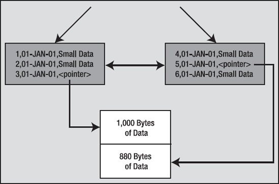
The gray boxes are the index entries, part of a larger index structure (in Chapter 11, you'll see a larger picture of what an index looks like). Briefly, the index structure is a tree, and the leaf blocks (where the data is stored) are, in effect, a doubly linked list to make it easier to traverse the nodes in order once we've found where we want to start in the index. The white box represents an OVERFLOW segment. This is where data that exceeds our PCTTHRESHOLD setting will be stored. Oracle will work backward from the last column up to but not including the last column of the primary key to find out what columns need to be stored in the overflow segment. In this example, the number column X and the date column Y will always fit in the index block. The last column, Z, is of varying length. When it is less than about 190 bytes or so (10 percent of a 2KB block is about 200 bytes; subtract 7 bytes for the date and 3 to 5 for the number), it will be stored on the index block. When it exceeds 190 bytes, Oracle will store the data for Z in the overflow segment and set up a pointer (a rowid, in fact) to it.

The other option is to use the INCLUDING clause. Here we are stating explicitly what columns we want stored on the index block and which should be stored in the overflow. Given a CREATE TABLE statement like this

ops$tkyte@ORA11GR2> create table iot
  2  (  x    int,
  3     y    date,
  4     z    varchar2(2000),
  5     constraint iot_pk primary key (x)
  6  )
  7  organization index
  8  including y
  9  overflow
 10  /
Table created.

what we can expect to find is illustrated in Figure 10-7.

Figure 10-7. IOT with OVERFLOW segment, INCLUDING clause

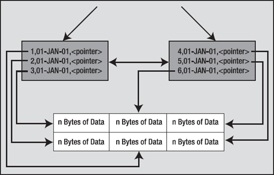
In this situation, regardless of the size of the data stored in it, Z will be stored out of line in the overflow segment.

Which is better then: PCTTHRESHOLD, INCLUDING, or some combination of both? It depends on your needs. If you have an application that always, or almost always, uses the first four columns of a table and rarely accesses the last five columns, using INCLUDING would be appropriate. You would include up to the fourth column and let the other five be stored out of line. At runtime, if you need them, the columns will be retrieved in much the same way as a migrated (also known as a chained) row would be. Oracle will read the head of the row, find the pointer to the rest of the row, and then read that. If, on the other hand, you cannot say that you almost always access these columns and hardly ever access those columns, you should give some consideration to PCTTHRESHOLD. Setting PCTTHRESHOLD is easy once you determine the number of rows you would like to store per index block on average. Suppose you wanted 20 rows per index block. Well, that means each row should be one-twentieth (5 percent). Your PCTTHRESHOLD would be 5, and each chunk of the row that stays on the index leaf block should consume no more than 5 percent of the block.

The last thing to consider with IOTs is indexing. You can have an index on IOTs themselves—sort of like having an index on an index. These are called secondary indexes. Normally, an index contains the physical address of the row it points to, the rowid. An IOT secondary index cannot do this; it must use some other way to address the row. This is because a row in an IOT can move around a lot, and it does not migrate in the way a row in a heap organized table would. A row in an IOT is expected to be at some position in the index structure, based on its primary key value; it will only be moving because the size and shape of the index itself is changing. (We'll cover more about how index structures are maintained in the next chapter, "Indexes".) To accommodate this, Oracle introduced a logical rowid. These logical rowids are based on the IOT's primary key. They may also contain a guess as to the current location of the row, although this guess is almost always wrong because after a short while, data in an IOT tends to move. The guess is the physical address of the row in the IOT when it was first placed into the secondary index structure. If the row in the IOT has to move to another block, the guess in the secondary index becomes stale. Therefore, an index on an IOT is slightly less efficient than an index on a regular table. On a regular table, an index access typically requires the I/O to scan the index structure and then a single read to read the table data. With an IOT, typically two scans are performed: one on the secondary structure and the other on the IOT itself. That aside, indexes on IOTs provide fast and efficient access to the data in the IOT using columns other than the primary key.

I generally find people's understanding of what a cluster is in Oracle to be inaccurate. Many people tend to confuse a cluster with a SQL Server or Sybase "clustered index." They are not the same. A cluster is a way to store a group of tables that share some common column(s) in the same database blocks and to store related data together on the same block. A clustered index in SQL Server forces the rows to be stored in sorted order according to the index key, similar to an IOT as just described. With a cluster, a single block of data may contain data from many tables. Conceptually, you are storing the data "prejoined." It can also be used with single tables where you are storing data together grouped by some column. For example, all of the employees in department 10 will be stored on the same block (or as few blocks as possible, if they all don't fit). It is not storing the data sorted—that is the role of the IOT. It is storing the data clustered by some key, but in a heap. So, department 100 might be right next to department 1, and very far away (physically on disk) from departments 101 and 99.

Graphically, you might think of it as shown in Figure 10-8. On the left side of the image, we are using conventional tables. EMP will be stored in its segment. DEPT will be stored on its own. They may be in different files and different tablespaces, and they are definitely in separate extents. On the right side of the image, we see what would happen if we clustered these two tables together. The square boxes represent database blocks. We now have the value 10 factored out and stored once. Then, all of the data from all of the tables in the cluster for department 10 is stored in that block. If all of the data for department 10 does not fit on the block, then additional blocks will be chained to the original block to contain the overflow, in the same fashion as the overflow blocks for an IOT.

Figure 10-8. Index clustered data

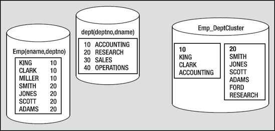
So, let's look at how we might go about creating a clustered object. Creating a cluster of tables in the object is straightforward. The definition of the storage of the object (PCTFREE, PCTUSED, INITIAL, and so on) is associated with the CLUSTER, not the tables. This makes sense since there will be many tables in the cluster, and they will be on the same block. Having different PCTFREEs would not make sense. Therefore, a CREATE CLUSTER statement looks a lot like a CREATE TABLE statement with a small number of columns (just the cluster key columns):

ops$tkyte@ORA11GR2> create cluster emp_dept_cluster
  2  ( deptno number(2) )
  3  size 1024
  4  /
Cluster created.

Here, we have created an index cluster (the other type being a hash cluster, which we'll look at in the next section "Index Clustered Tables Wrap-up"). The clustering column for this cluster will be the DEPTNO column. The columns in the tables do not have to be called DEPTNO but they must be NUMBER(2) to match this definition. We have, on the cluster definition, a SIZE 1024 option. This is used to tell Oracle that we expect about 1,024 bytes of data to be associated with each cluster key value. Oracle will use that to compute the maximum number of cluster keys that could fit per block. Given that we have an 8KB block size, Oracle will fit up to seven cluster keys (but maybe less if the data is larger than expected) per database block. For example, the data for departments 10, 20, 30, 40, 50, 60, and 70 would tend to go onto one block, and as soon as we insert department 80, a new block will be used. This does not mean that the data is stored in a sorted manner; it just means that if we inserted the departments in that order, they would naturally tend to be put together. If we inserted the departments in the order 10, 80, 20, 30, 40, 50, 60, and then 70, the final department (70) would tend to be on the newly added block. As we'll see below, both the size of the data and the order in which the data is inserted will affect the number of keys we can store per block.

The SIZE parameter therefore controls the maximum number of cluster keys per block. It is the single largest influence on the space utilization of our cluster. Set the size too high, and we'll get very few keys per block and we'll use more space than we need. Set the size too low, and we'll get excessive chaining of data, which offsets the purpose of the cluster to store all of the data together on a single block. It is the most important parameter for a cluster.

Now for the cluster index on our cluster. We need to index the cluster before we can put data in it. We could create tables in the cluster right now, but we're going to create and populate the tables simultaneously, and we need a cluster index before we can have any data. The cluster index's job is to take a cluster key value and return the block address of the block that contains that key. It is a primary key, in effect, where each cluster key value points to a single block in the cluster itself. So, when we ask for the data in department 10, Oracle will read the cluster key, determine the block address for that, and then read the data. The cluster key index is created as follows:

ops$tkyte@ORA11GR2> create index emp_dept_cluster_idx
  2  on cluster emp_dept_cluster
  3  /
Index created.

It can have all of the normal storage parameters of an index and can be stored in another tablespace. It is just a regular index, so it can be on multiple columns; it just happens to index into a cluster and can also include an entry for a completely null value (see Chapter 11 for the reason why this is interesting). Note that we do not specify a list of columns in this CREATE INDEX statement—that is derived from the CLUSTER definition itself. Now we are ready to create our tables in the cluster:

ops$tkyte@ORA11GR2> create table dept
  2  ( deptno number(2) primary key,
  3    dname  varchar2(14),
  4    loc    varchar2(13)
  5  )
  6  cluster emp_dept_cluster(deptno)
  7  /
Table created.

ops$tkyte@ORA11GR2> create table emp
  2  ( empno    number primary key,
  3    ename    varchar2(10),
  4    job      varchar2(9),
  5    mgr      number,
  6    hiredate date,
  7    sal      number,
  8    comm     number,
  9    deptno number(2) references dept(deptno)
 10  )
 11  cluster emp_dept_cluster(deptno)
 12  /
Table created.

Here, the only difference from a normal table is that we used the CLUSTER keyword and told Oracle which column of the base table will map to the cluster key in the cluster itself. Remember, the cluster is the segment here, therefore this table will never have segment attributes such as TABLESPACE, PCTFREE, and so on—they are attributes of the cluster segment, not the table we just created. We can now load them up with the initial set of data:

ops$tkyte%ORA11GR2> insert into dept
  2  ( deptno, dname, loc )
  3  select deptno+r, dname, loc
  4    from scott.dept,

5        (select level r from dual connect by level < 10);

36 rows created.

ops$tkyte%ORA11GR2> insert into emp
  2  (empno, ename, job, mgr, hiredate, sal, comm, deptno)
  3  select rownum, ename, job, mgr, hiredate, sal, comm, deptno+r
  4    from scott.emp,
  5        (select level r from dual connect by level < 10);

126 rows created.

Now that the data is loaded, let's look at the organization of it on disk. We'll use the DBMS_ROWID package to peek into the rowid and see what blocks data is stored on. Let's first look at the DEPT table and see how many DEPT rows per block we have:

ops$tkyte%ORA11GR2> select min(count(*)), max(count(*)), avg(count(*))
  2    from dept
  3   group by dbms_rowid.rowid_block_number(rowid)
  4  /

MIN(COUNT(*)) MAX(COUNT(*)) AVG(COUNT(*))
------------- ------------- -------------
            1             7             6

So, even though we loaded DEPT first—and the DEPT rows are very small (hundreds of them could fit on an 8k block normally)—we find that the maximum number of DEPT rows on a block in this table is only seven. That fits in with what we anticipated above when we set the SIZE to 1024. We estimated that with an 8k block and 1024 bytes of data per cluster key for the combined EMP and DEPT records, we would see approximately seven unique cluster key values per block, and that is exactly what we are seeing here. Next, let's look at the EMP and DEPT table together. We'll look at the rowids of each and compare the block numbers after joining by DEPTNO. If the block numbers are the same, we'll know that the EMP row and the DEPT row are stored on the same physical database block together if they differ we'll know they are not. In this case, we observe that all of our data is perfectly stored. There are no cases where a record for the EMP table is stored on a block separate from its corresponding DEPT record:

ops$tkyte%ORA11GR2> select *
  2    from (
  3  select dept_blk, emp_blk,
  4         case when dept_blk <> emp_blk then '*' end flag,
  5             deptno

6    from (
  7  select dbms_rowid.rowid_block_number(dept.rowid) dept_blk,
  8         dbms_rowid.rowid_block_number(emp.rowid) emp_blk,
  9         dept.deptno
 10    from emp, dept
 11   where emp.deptno = dept.deptno
 12         )
 13             )
 14   where flag = '*'
 15   order by deptno
 16  /
no rows selected

That was exactly our goal—to get every row in the EMP table stored on the same block as the corresponding DEPT row. But what would have happened if we estimated incorrectly, what if 1024 was insufficient? What if some of our departments were close to 1024 and others exceeded that value? Then, obviously, the data could not fit on the same block and we'd have to place some of the EMP records on a block separate from the DEPT record. We can see this easily by resetting our example above (I'm starting with the tables as they were before the load above, right after creating them). When I load this time, we'll load every EMP record eight times, to multiply the number of employee records per each department:

ops$tkyte%ORA11GR2> insert into dept
  2  ( deptno, dname, loc )
  3  select deptno+r, dname, loc
  4    from scott.dept,
  5        (select level r from dual connect by level < 10);

36 rows created.

ops$tkyte%ORA11GR2> insert into emp
  2  (empno, ename, job, mgr, hiredate, sal, comm, deptno)
  3  select rownum, ename, job, mgr, hiredate, sal, comm, deptno+r
  4    from scott.emp,
  5        (select level r from dual connect by level < 10),
  6            (select level r2 from dual connect by level < 8);

882 rows created.

ops$tkyte%ORA11GR2>
ops$tkyte%ORA11GR2> select min(count(*)), max(count(*)), avg(count(*))
  2    from dept
  3   group by dbms_rowid.rowid_block_number(rowid)
  4  /

MIN(COUNT(*)) MAX(COUNT(*)) AVG(COUNT(*))
------------- ------------- -------------
            1             7             6

So far, it looks just like the prior example, but when we compare the blocks the EMP records are on to the blocks the DEPT records are on

ops$tkyte%ORA11GR2> select *
  2    from (
  3  select dept_blk, emp_blk,
  4         case when dept_blk <> emp_blk then '*' end flag,
  5             deptno
  6    from (
  7  select dbms_rowid.rowid_block_number(dept.rowid) dept_blk,
  8         dbms_rowid.rowid_block_number(emp.rowid) emp_blk,
  9         dept.deptno
 10    from emp, dept
 11   where emp.deptno = dept.deptno
 12         )
 13             )
 14   where flag = '*'
 15   order by deptno
 16  /

  DEPT_BLK    EMP_BLK F     DEPTNO
---------- ---------- - ----------
       523        554 *         12
       523        554 *         12
...
       526        554 *         39
       526        554 *         39

45 rows selected.

we can see there are 45 out of 882 EMP rows on a block separate and distinct from the block their corresponding DEPTNO is on in the DEPT table. Given that we undersized the cluster (the SIZE parameter was too small given our real life data), we could recreate it with a cluster SIZE of 1200 and then we would discover

ops$tkyte%ORA11GR2> select min(count(*)), max(count(*)), avg(count(*))
  2    from dept
  3   group by dbms_rowid.rowid_block_number(rowid)
  4  /

MIN(COUNT(*)) MAX(COUNT(*)) AVG(COUNT(*))
------------- ------------- -------------
            6             6             6

ops$tkyte%ORA11GR2>
ops$tkyte%ORA11GR2> select *
  2    from (
  3  select dept_blk, emp_blk,
  4         case when dept_blk <> emp_blk then '*' end flag,
  5             deptno
  6    from (
  7  select dbms_rowid.rowid_block_number(dept.rowid) dept_blk,
  8         dbms_rowid.rowid_block_number(emp.rowid) emp_blk,
  9         dept.deptno
 10    from emp, dept
 11   where emp.deptno = dept.deptno
 12         )

13             )
 14   where flag = '*'
 15   order by deptno
 16  /

no rows selected

we only stored six DEPTNO values per block now, leaving sufficient room for all of the EMP data to be stored on the same block with their corresponding DEPT records.

Here is a bit of puzzle to amaze and astound your friends with. Many people mistakenly believe a rowid uniquely identifies a row in a database, and that given a rowid you can tell what table the row came from. In fact, you cannot. You can and will get duplicate rowids from a cluster. For example, after executing the preceding code you should find:

ops$tkyte%ORA11GR2> select rowid from emp
  2  intersect
  3  select rowid from dept;

ROWID
------------------
AAAWy1AAEAAAAILAAA
AAAWy1AAEAAAAILAAB
...
AAAWy1AAEAAAAIsAAD
AAAWy1AAEAAAAIsAAE
AAAWy1AAEAAAAIsAAF

36 rows selected.

Every rowid assigned to the rows in DEPT has been assigned to the rows in EMP as well. That is because it takes a table and row ID to uniquely identify a row. The rowid pseudo-column is unique only within a table.

I also find that many people believe the cluster object to be an esoteric object that no one really uses—everyone just uses normal tables. In fact, you use clusters every time you use Oracle. Much of the data dictionary is stored in various clusters, for example:

sys%ORA11GR2> break on cluster_name
sys%ORA11GR2> select cluster_name, table_name
  2    from user_tables
  3   where cluster_name is not null
  4   order by 1;

CLUSTER_NAME                   TABLE_NAME
------------------------------ ------------------------------
C_COBJ#                        CDEF$
                               CCOL$
C_FILE#_BLOCK#                 SEG$
                               UET$
C_MLOG#                        MLOG$
                               SLOG$
C_OBJ#                         SUBCOLTYPE$
                               NTAB$
                               REFCON$

OPQTYPE$
                               ICOLDEP$
                               VIEWTRCOL$
                               LIBRARY$
                               ASSEMBLY$
                               ATTRCOL$
                               TYPE_MISC$
                               COLTYPE$
                               LOB$
                               TAB$
                               CLU$
                               COL$
                               ICOL$
                               IND$
C_OBJ#_INTCOL#                 HISTGRM$
C_RG#                          RGROUP$
                               RGCHILD$
C_TOID_VERSION#                PARAMETER$
                               RESULT$
                               METHOD$
                               ATTRIBUTE$
                               COLLECTION$
                               TYPE$
C_TS#                          TS$
                               FET$
C_USER#                        TSQ$
                               USER$
SMON_SCN_TO_TIME_AUX           SMON_SCN_TIME

37 rows selected.

As you can see, most of the object-related data is stored in a single cluster (the C_OBJ# cluster): 16 tables sharing the same block. It is mostly column-related information stored there, so all of the information about the set of columns of a table or index is stored physically on the same block. This makes sense, as when Oracle parses a query, it wants to have access to the data for all of the columns in the referenced table. If this data were spread all over the place, it would take a while to get it together. Here, it is on a single block typically and readily available.

When would you use a cluster? It is easier perhaps to describe when not to use one:

So, if you have data that is mostly read (that does not mean "never written"; it is perfectly OK to modify cluster tables) and read via indexes, either the cluster key index or other indexes you put on the tables in the cluster, and join this information together frequently, a cluster would be appropriate. Look for tables that are logically related and always used together, like the people who designed the Oracle data dictionary when they clustered all column-related information together.

Hash clustered tables are very similar in concept to the index clustered tables just described with one main exception: the cluster key index is replaced with a hash function. The data in the table is the index; there is no physical index. Oracle will take the key value for a row, hash it using either an internal function or one you supply, and use that to figure out where the data should be on disk. One side effect of using a hashing algorithm to locate data, however, is that you cannot range scan a table in a hash cluster without adding a conventional index to the table. In an index cluster, the query

select * from emp where deptno between 10 and 20

would be able to make use of the cluster key index to find these rows. In a hash cluster, this query would result in a full table scan unless you had an index on the DEPTNO column. Only exact equality searches (including IN lists and subqueries) may be made on the hash key without using an index that supports range scans.

In a perfect world, with nicely distributed hash key values and a hash function that distributes them evenly over all of the blocks allocated to the hash cluster, we can go straight from a query to the data with one I/O. In the real world, we will end up with more hash key values hashing to the same database block address than fit on that block. This will result in Oracle having to chain blocks together in a linked list to hold all of the rows that hash to this block. Now, when we need to retrieve the rows that match our hash key, we might have to visit more than one block.

Like a hash table in a programming language, hash tables in the database have a fixed size. When you create the table, you must determine the number of hash keys your table will have, forever. That does not limit the amount of rows you can put in there.

In Figure 10-9, we can see a graphical representation of a hash cluster with table EMP created in it. When the client issues a query that uses the hash cluster key in the predicate, Oracle will apply the hash function to determine which block the data should be in. It will then read that one block to find the data. If there have been many collisions, or the SIZE parameter to the CREATE CLUSTER was underestimated, Oracle will have allocated overflow blocks that are chained off the original block.

Figure 10-9. Depiction of a hash cluster

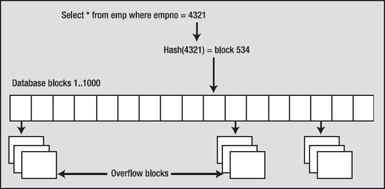
When you create a hash cluster, you'll use the same CREATE CLUSTER statement you used to create the index cluster with different options. You'll just be adding a HASHKEYS option to it to specify the size of the hash table. Oracle will take your HASHKEYS value and round it up to the nearest prime number; the number of hash keys will always be a prime. Oracle will then compute a value based on the SIZE parameter multiplied by the modified HASHKEYS value. It will allocate at least that much space in bytes for the cluster. This is a big difference from the preceding index cluster, which dynamically allocates space as it needs it. A hash cluster pre-allocates enough space to hold (HASHKEYS/trunc(blocksize/SIZE)) bytes of data. For example, if you set your SIZE to 1,500 bytes and you have a 4KB block size, Oracle will expect to store two keys per block. If you plan on having 1,000 HASHKEYs, Oracle will allocate 500 blocks.

It is interesting to note that unlike a conventional hash table in a computer language, it is OK to have hash collisions—in fact, it is desirable in many cases. If you take the same DEPT/EMP example from earlier, you could set up a hash cluster based on the DEPTNO column. Obviously, many rows will hash to the same value, and you expect them to (they have the same DEPTNO). This is what the cluster is about in some respects: clustering like data together. This is why Oracle asks you to specify the HASHKEYs (how many department numbers you anticipate over time) and SIZE (what the size of the data is that will be associated with each department number). It allocates a hash table to hold HASHKEY number of departments of SIZE bytes each. What you do want to avoid is unintended hash collisions. It is obvious that if you set the size of the hash table to 1,000 (really 1,009, since the hash table size is always a prime number and Oracle rounds up for you), and you put 1,010 departments in the table, there will be at least one collision (two different departments hashing to the same value). Unintended hash collisions are to be avoided, as they add overhead and increase the probability of block chaining occurring.

To see what sort of space hash clusters take, we'll use a small utility stored procedure SHOW_SPACE (for details on this procedure, see the "Setting Up Your Environment" section at the beginning of the book) that we'll use in this chapter and in the next chapter. This routine just uses the DBMS_SPACE-supplied package to get details about the storage used by segments in the database.

Now, if we issue a CREATE CLUSTER statement, such as the following, we can see the storage it allocated:

ops$tkyte%ORA11GR2> create cluster hash_cluster
  2  ( hash_key number )
  3  hashkeys 1000
  4  size 8192

5  tablespace mssm
  6  /
Cluster created.

ops$tkyte%ORA11GR2> exec show_space( 'HASH_CLUSTER', user, 'CLUSTER' )
Free Blocks.............................               0
Total Blocks............................           1,024
Total Bytes.............................       8,388,608
Total MBytes............................               8
Unused Blocks...........................              14
Unused Bytes............................         114,688
Last Used Ext FileId....................               7
Last Used Ext BlockId...................           1,024
Last Used Block.........................             114

PL/SQL procedure successfully completed.

We can see that the total number of blocks allocated to the table is 1,024. Fourteen of these blocks are unused (free). One block goes to table overhead to manage the extents. Therefore, 1,009 blocks are under the HWM of this object, and these are used by the cluster. The prime 1,009 just happens to be the next largest prime over 1,000, and since the block size is 8KB, we can see that Oracle did in fact allocate and format 1009 blocks for us. The figure is a little higher than this due to the way extents are rounded and/or by using locally managed tablespaces with uniformly sized extents.

This example points out one of the issues with hash clusters you need to be aware of. Normally, if we create an empty table, the number of blocks under the HWM for that table is 0. If we full scan it, it reaches the HWM and stops. With a hash cluster, the tables will start out big and will take longer to create, as Oracle must initialize each block, an action that normally takes place as data is added to the table. They have the potential to have data in their first block and their last block, with nothing in between. Full scanning a virtually empty hash cluster will take as long as full scanning a full hash cluster. This is not necessarily a bad thing; we built the hash cluster to have very fast access to the data by a hash key lookup. We did not build it to full scan it frequently.

Now we can start placing tables into the hash cluster in the same fashion we did with index clusters:

Ops$tkyte@ORA11GR2> create table hashed_table
  2  ( x number, data1 varchar2(4000), data2 varchar2(4000) )
  3  cluster hash_cluster(x);
Table created.

To see the difference a hash cluster can make, I set up a small test. I created a hash cluster, loaded some data in it, copied this data to a regular table with a conventional index on it, and then did random reads on each table (the same "random" reads on each). Using runstats, SQL_TRACE, and TKPROF, I was able to determine the characteristics of each. The following is the setup I performed, followed by the analysis:

ops$tkyte%ORA11GR2> create cluster hash_cluster
  2  ( hash_key number )
  3  hashkeys 75000
  4  size 150
  5  /
Cluster created.

ops$tkyte%ORA11GR2> create table t_hashed
  2  cluster hash_cluster(object_id)

3  as
  4  select *
  5    from all_objects
  6  /
Table created.

ops$tkyte%ORA11GR2> alter table t_hashed add constraint
  2  t_hashed_pk primary key(object_id)
  3  /
Table altered.

ops$tkyte%ORA11GR2> begin
  2    dbms_stats.gather_table_stats( user, 'T_HASHED' );
  3  end;
  4  /
PL/SQL procedure successfully completed.

I created the hash cluster with a SIZE of 150 bytes. This is because I determined the average row size for a row in my table would be about 100 bytes, but would vary up and down based on the data with many rows coming in at around 150 bytes. I then created and populated a table in that cluster as a copy of ALL_OBJECTS.

Next, I created the conventional clone of the table:

ops$tkyte%ORA11GR2> create table t_heap
  2  as
  3  select *
  4    from t_hashed
  5  /
Table created.

ops$tkyte%ORA11GR2> alter table t_heap add constraint
  2  t_heap_pk primary key(object_id)
  3  /
Table altered.

ops$tkyte%ORA11GR2> begin
  2     dbms_stats.gather_table_stats( user, 'T_HEAP' );
  3  end;
  4  /
PL/SQL procedure successfully completed.

Now, all I needed was some random data to pick rows from each of the tables with. To achieve that, I simply selected all of the OBJECT_IDs into an array and had them sorted randomly, to hit the table all over in a scattered fashion. I used a PL/SQL package to define and declare the array and a bit of PL/SQL code to prime the array, to fill it up:

ops$tkyte%ORA11GR2> create or replace package state_pkg
  2  as
  3      type array is table of t_hashed.object_id%type;
  4      g_data array;
  5  end;
  6  /

Package created.

ops$tkyte%ORA11GR2> begin
  2      select object_id bulk collect into state_pkg.g_data
  3        from t_hashed
  4       order by dbms_random.random;
  5  end;
  6  /
PL/SQL procedure successfully completed.

To see the work performed by each, I used the following block of code (if you replace occurrences of the word HEAP with HASHED, you have the other block of code you need to test against):

ops$tkyte%ORA11GR2> declare
  2      l_rec t_heap%rowtype;
  3  begin
  4      for i in 1 .. state_pkg.g_data.count
  5      loop
  6          select * into l_rec from t_heap
  7          where object_id = state_pkg.g_data(i);
  8      end loop;
  9  end;
 10  /
PL/SQL procedure successfully completed.

Next, I ran the preceding block of code three times (and the copy of that block of code where HEAP is replaced with HASHED as well). The first run was to warm up the system, to get any hard parses out of the way. The second time I ran the blocks of code, I used runstats to see the material differences between the two: running first the hashed implementation and then the heap. The third time I ran the blocks of code, I did so with SQL_TRACE enabled so I could see a TKPROF report. The runstats run reported the following:

ops$tkyte@ORA11GR2> exec runstats_pkg.rs_stop(10000);
Run1 ran in 344 cpu hsecs
Run2 ran in 344 cpu hsecs
run 1 ran in 100.00% of the time

Name                                  Run1        Run2        Diff
STAT...Cached Commit SCN refer      31,638           0     −31,638
LATCH.cache buffers chains         144,396     216,415      72,019
STAT...rows fetched via callba           0      72,081      72,081
STAT...cluster key scan block       72,081           0     −72,081
STAT...table fetch by rowid              0      72,081      72,081
STAT...no work - consistent re      72,081           0     −72,081
STAT...index fetch by key                0      72,081      72,081
STAT...cluster key scans            72,081           0     −72,081
STAT...consistent gets from ca      72,090           9     −72,081
STAT...buffer is not pinned co      72,081     216,243     144,162
STAT...consistent gets              72,098     216,260     144,162
STAT...consistent gets from ca      72,098     216,260     144,162
STAT...session logical reads        72,129     216,293     144,164
STAT...consistent gets - exami           8     216,251     216,243

Run1 latches total versus runs -- difference and pct
Run1        Run2        Diff       Pct
149,837     223,287      73,450     67.11%

Now, these two simulations ran in about the same amount of time by the CPU clock. The material difference to note, however, is the large reduction in cache buffers chains latches. The first implementation (hashed) used significantly fewer, meaning the hashed implementation should scale better in a read-intensive environment, since it needs fewer resources that require some level of serialization. This was due entirely to the fact that the I/O needed by the hashed implementation was significantly reduced over the HEAP table—you can see the statistic consistent gets in that report bears this out. The TKPROF shows it even more clearly:

SELECT * FROM T_HASHED WHERE OBJECT_ID = :B1

call     count       cpu    elapsed       disk      query    current        rows
------- ------  -------- ---------- ---------- ---------- ----------  ----------
Parse        1      0.00       0.00          0          0          0           0
Execute  72081     10.20      10.36          0          2          0           0
Fetch    72081      1.73       1.69          0      72081          0       72081
------- ------  -------- ---------- ---------- ---------- ----------  ----------
total   144163     11.94      12.06          0      72083          0       72081

Rows     Row Source Operation
-------  ---------------------------------------------------
      1  TABLE ACCESS HASH T_HASHED (cr=1 pr=0 pw=0 time=0 us)
********************************************************************************
SELECT * FROM T_HEAP WHERE OBJECT_ID = :B1

call     count       cpu    elapsed       disk      query    current        rows
------- ------  -------- ---------- ---------- ---------- ----------  ----------
Parse        1      0.00       0.00          0          0          0           0
Execute  72080     10.55      10.84          0          0          0           0
Fetch    72080      1.80       1.85          0     216240          0       72080
------- ------  -------- ---------- ---------- ---------- ----------  ----------
total   144161     12.36      12.70          0     216240          0       72080

Rows     Row Source Operation
-------  ---------------------------------------------------
      1  TABLE ACCESS BY INDEX ROWID T_HEAP (cr=3 pr=0 pw=0 time=0 us cost=2 si...)
      1   INDEX UNIQUE SCAN T_HEAP_PK (cr=2 pr=0 pw=0 time=0 us cost=1 size=0 ...)

The HASHED implementation simply converted the OBJECT_ID passed into the query into a FILE/BLOCK to be read and read it—no index. The HEAP table, however, had to do two I/Os on the index for each row. The cr=2 in the TKPROF Row Source Operation line shows us exactly how many consistent reads were done against the index. Each time I looked up OBJECT_ID = :B1, Oracle had to get the root block of the index and then find the leaf block containing the location of that row. Then, I had to take the leaf block information, which included the ROWID of that row, and access that row in the table for a third I/O. The HEAP table did three times the I/O of the HASHED implementation.

The points of interest here are as follows:

This last point is the important one. When working with computers, it is all about resources and their utilization. If we are I/O bound and perform queries that do lots of keyed reads like I just did, a hash cluster may improve performance. If we are already CPU bound, a hash cluster may possibly decrease performance since it needs more CPU horsepower to hash. However, if the extra CPU we are burning is due to spinning on cache buffers chains latches, the hash cluster could significantly reduce the CPU needed. This is one of the major reasons why rules of thumb do not work on real-world systems: what works for you might not work for others in similar but different conditions.

There is a special case of a hash cluster called a single table hash cluster. This is an optimized version of the general hash cluster we've already looked at. It supports only one table in the cluster at a time (you have to DROP the existing table in a single table hash cluster before you can create another). Additionally, if there is a one-to-one mapping between hash keys and data rows, the access to the rows is somewhat faster as well. These hash clusters are designed for those occasions when you want to access a table by primary key and do not care to cluster other tables with it. If you need fast access to an employee record by EMPNO, a single table hash cluster might be called for. I did the preceding test on a single table hash cluster as well and found the performance to be even better than just a hash cluster. You could even go a step further with this example and take advantage of the fact that Oracle will allow you to write your own specialized hash function (instead of using the default one provided by Oracle). You are limited to using only the columns available in the table, and you may use only the Oracle built-in functions (e.g., no PL/SQL code) when writing these hash functions. By taking advantage of the fact that OBJECT_ID is a number between 1 and 75,000 in the preceding example, I made my hash function simply be the OBJECT_ID column itself. In this fashion, I am guaranteed to never have a hash collision. Putting it all together, I'll create a single table hash cluster with my own hash function via:

ops$tkyte@ORA11GR2> create cluster hash_cluster
  2  ( hash_key number(10) )
  3  hashkeys 75000
  4  size 150
  5  single table
  6  hash is HASH_KEY
  7  /
Cluster created.

I've simply added the key words SINGLE TABLE to make it a single table hash cluster. My HASH IS function is just the HASH_KEY cluster key in this case. This is a SQL function, so I could have used trunc(mod(hash_key/324+278,555)/abs(hash_key+1)) if I wanted (not that this is a good hash function—it just demonstrates that we can use a complex function there if we wish). I used a NUMBER(10) instead of just a number. Since the hash value must be an integer, it cannot have any fractional components. Then, I create the table in that cluster

ops$tkyte@ORA11GR2> create table t_hashed
  2  cluster hash_cluster(object_id)
  3  as
  4  select OWNER, OBJECT_NAME, SUBOBJECT_NAME,
  5         cast( OBJECT_ID as number(10) ) object_id,
  6         DATA_OBJECT_ID, OBJECT_TYPE, CREATED,
  7         LAST_DDL_TIME, TIMESTAMP, STATUS, TEMPORARY,
  8         GENERATED, SECONDARY

9    from all_objects
 10  /
Table created.

to build the hashed table. Note the use of the CAST built-in function to make the datatype of OBJECT_ID be what it must be. I ran the test as before (three runs of each block), and this time the runstats output was consistently even more positive:

Run1 ran in 299 cpu hsecs
Run2 ran in 344 cpu hsecs
run 1 ran in 86.92% of the time

Name                                  Run1        Run2        Diff
STAT...Cached Commit SCN refer      30,671           0     −30,671
STAT...index fetch by key                0      72,081      72,081
STAT...cluster key scans            72,081           0     −72,081
STAT...table fetch by rowid              0      72,093      72,093
STAT...session pga memory                0    −131,072    −131,072
LATCH.cache buffers chains          77,000     216,458     139,458
STAT...session logical reads        72,924     216,308     143,384
STAT...consistent gets from ca      72,864     216,272     143,408
STAT...consistent gets              72,864     216,272     143,408
STAT...buffer is not pinned co      72,855     216,267     143,412
STAT...consistent gets - exami      68,956     216,250     147,294

Run1 latches total versus runs -- difference and pct
Run1        Run2        Diff       Pct
82,489     225,414     142,925     36.59%

PL/SQL procedure successfully completed.

This single table hash cluster required even less latching into the buffer cache to process (it can stop looking for data sooner, and it has more information). As a result, the TKPROF report shows a measurable decrease in CPU utilization this time around:

SELECT * FROM T_HASHED WHERE OBJECT_ID = :B1

call     count       cpu    elapsed       disk      query    current        rows
------- ------  -------- ---------- ---------- ---------- ----------  ----------
Parse        1      0.00       0.00          0          0          0           0
Execute  72080      9.66      10.34          0          2          0           0
Fetch    72080      1.31       1.29          0      72854          0       72080
------- ------  -------- ---------- ---------- ---------- ----------  ----------
total   144161     10.97      11.64          0      72856          0       72080

Rows     Row Source Operation
-------  ---------------------------------------------------
      1  TABLE ACCESS HASH T_HASHED (cr=1 pr=0 pw=0 time=0 us)
********************************************************************************
SELECT * FROM T_HEAP WHERE OBJECT_ID = :B1

call     count       cpu    elapsed       disk      query    current        rows
------- ------  -------- ---------- ---------- ---------- ----------  ----------
Parse        1      0.00       0.00          0          0          0           0

Execute  72081     10.42      10.49          0          0          0           0
Fetch    72081      1.77       1.78          0     216243          0       72081
------- ------  -------- ---------- ---------- ---------- ----------  ----------
total   144163     12.19      12.27          0     216243          0       72081

Sorted hash clusters are new in Oracle 10g. They combine the qualities of the hash cluster just described with those of an IOT. They are most appropriate when you constantly retrieve data using a query similar to this:

Select *
  From t
 Where KEY=:x
 Order by SORTED_COLUMN

That is, you retrieve the data by some key and need that data ordered by some other column. Using a sorted hash cluster, Oracle can return the data without performing a sort at all. It accomplishes this by storing the data upon insert in sorted order physically—by key. Suppose you have a customer order table:

ops$tkyte@ORA11GR2> select cust_id, order_dt, order_number
  2   from cust_orders
  3   order by cust_id, order_dt;

CUST_ID ORDER_DT                     ORDER_NUMBER
------- ---------------------------- ------------
      1 31-MAR-05 09.13.57.000000 PM        21453
        11-APR-05 08.30.45.000000 AM        21454
        28-APR-05 06.21.09.000000 AM        21455
      2 08-APR-05 03.42.45.000000 AM        21456
        19-APR-05 08.59.33.000000 AM        21457
        27-APR-05 06.35.34.000000 AM        21458
        30-APR-05 01.47.34.000000 AM        21459

7 rows selected.

The table is stored in a sorted hash cluster, whereby the HASH key is CUST_ID and the field to sort on is ORDER_DT. Graphically, it might look like Figure 10-10, where 1, 2, 3, 4, ... represent the records stored sorted on each block.

Figure 10-10. Depiction of a sorted hash cluster

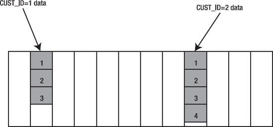
Creating a sorted hash cluster is much the same as the other clusters. To set up a sorted hash cluster capable of storing the above data, we could use the following:

ops$tkyte@ORA11GR2> CREATE CLUSTER shc
  2  (
  3     cust_id     NUMBER,
  4     order_dt    timestamp SORT
  5  )
  6  HASHKEYS 10000
  7  HASH IS cust_id
  8  SIZE  8192
  9  /
Cluster created.

We've introduced a new keyword here: SORT. When we created the cluster, we identified the HASH IS CUST_ID and we added an ORDER_DT of type timestamp with the keyword SORT. This means the data will be located by CUST_ID (where CUST_ID=:x) and physically retrieved sorted by ORDER_DT. Technically, it really means we'll store some data that will be retrieved via a NUMBER column and sorted by the TIMESTAMP. The column names here are not relevant, as they were not in the B*Tree or HASH clusters, but convention would have us name them after what they represent.

The CREATE TABLE statement for our CUST_ORDERS table would look like this:

ops$tkyte@ORA11GR2> CREATE TABLE cust_orders
  2  (  cust_id       number,
  3     order_dt      timestamp SORT,
  4     order_number  number,
  5     username      varchar2(30),
  6     ship_addr     number,
  7     bill_addr     number,
  8     invoice_num   number
  9  )
 10  CLUSTER shc ( cust_id, order_dt )
 11  /
Table created.

We've mapped the CUST_ID column of this table to the hash key for the sorted hash cluster and the ORDER_DT column to the SORT column. We can observe using AUTOTRACE in SQL*Plus that the normal sort operations we expect are missing when accessing the sorted hash cluster:

ops$tkyte@ORA11GR2> set autotrace traceonly explain
ops$tkyte@ORA11GR2> variable x number
ops$tkyte@ORA11GR2> select cust_id, order_dt, order_number
  2    from cust_orders
  3   where cust_id = :x
  4   order by order_dt;

Execution Plan
----------------------------------------------------------
   0      SELECT STATEMENT Optimizer=ALL_ROWS (Cost=0 Card=4 Bytes=76)
   1    0   TABLE ACCESS (HASH) OF 'CUST_ORDERS' (CLUSTER (HASH))

ops$tkyte@ORA11GR2> select job, hiredate, empno
  2    from scott.emp

3   where job = 'CLERK'
  4   order by hiredate;

Execution Plan
----------------------------------------------------------
   0      SELECT STATEMENT Optimizer=ALL_ROWS (Cost=3 Card=3 Bytes=60)
   1    0   SORT (ORDER BY) (Cost=3 Card=3 Bytes=60)
   2    1     TABLE ACCESS (BY INDEX ROWID) OF 'EMP' (TABLE) (Cost=2 Card=3 ...
   3    2       INDEX (RANGE SCAN) OF 'JOB_IDX' (INDEX) (Cost=1 Card=3)

ops$tkyte@ORA11GR2> set autotrace off

I added the query against the normal SCOTT.EMP table (after indexing the JOB column for this demonstration) to compare what we normally expect to see: the SCOTT.EMP query plan versus what the sorted hash cluster can do for us when we want to access the data in a FIFO mode (like a queue). As you can see, the sorted hash cluster has one step: it takes the CUST_ID=:X, hashes the input, finds the first row, and just starts reading the rows, as they are in order already. The regular table is much different: it finds all of the JOB='CLERK' rows (which could be anywhere in that heap table), sorts them, and then returns the first one.

So, the sorted hash cluster has all the retrieval aspects of the hash cluster, in that it can get to the data without having to traverse an index, and many of the features of the IOT, in that the data will be sorted within that key by some field of your choice. This data structure works well when the input data arrives in order by the sort field, by key. That is, over time the data arrives in increasing sort order for any given key value. Stock information fits this requirement as an example. Every night you get a new file full of stock symbols, the date (the date would be the sort key and the stock symbol would be the hash key), and related information. You receive and load this data in sort key order. The stock data for stock symbol ORCL for yesterday does not arrive after today—you would load yesterday's value, and then today's value, and later tomorrow's value. If the information arrives randomly (not in sort order), this data structure quickly breaks down during the insert process, as much data has to be moved to put the rows physically in order on disk. A sorted hash cluster is not recommended in that case (an IOT, on the other hand, could well be useful for that data).

When considering using this structure, you should employ the same considerations from the hash cluster section, in addition to the constraint that the data should arrive sorted for each key value over time.

Nested tables are part of the object-relational extensions to Oracle. A nested table, one of the two collection types in Oracle, is very similar to a child table in a traditional parent/child table pair in the relational model. It is an unordered set of data elements, all of the same data type, which could be either a built-in data type or an object data type. It goes one step further, however, since it is designed to give the illusion that each row in the parent table has its own child table. If there are 100 rows in the parent table, then there are virtually 100 nested tables. Physically, there is only the single parent and the single child table. There are large syntactic and semantic differences between nested tables and parent/child tables as well, and we'll look at those in this section.

There are two ways to use nested tables. One is in your PL/SQL code as a way to extend the PL/SQL language. The other is as a physical storage mechanism for persistent storage of collections. I use them in PL/SQL all of the time, but I have never used them as a permanent storage mechanism.

In this section, I'll briefly introduce the syntax to create, query, and modify nested tables. Then we'll look at some of the implementation details and what is important to know about how Oracle really stores nested tables.

ops$tkyte@ORA11GR2> create table dept
  2  (deptno number(2) primary key,
  3   dname     varchar2(14),
  4   loc       varchar2(13)
  5  );
Table created.

ops$tkyte@ORA11GR2> create table emp
  2  (empno       number(4) primary key,
  3   ename       varchar2(10),
  4   job         varchar2(9),
  5   mgr         number(4) references emp,
  6   hiredate    date,
  7   sal         number(7, 2),
  8   comm        number(7, 2),
  9   deptno      number(2) references dept
 10  );
Table created.

ops$tkyte%ORA11GR2> create or replace type emp_type
  2  as object
  3  (empno       number(4),
  4   ename       varchar2(10),
  5   job         varchar2(9),
  6   mgr         number(4),
  7   hiredate    date,
  8   sal         number(7, 2),
  9   comm        number(7, 2)
 10  );
 11  /
Type created.

ops$tkyte%ORA11GR2> create or replace type emp_tab_type
  2  as table of emp_type
  3  /
Type created.

ops$tkyte%ORA11GR2> create table dept_and_emp
  2  (deptno number(2) primary key,
  3   dname     varchar2(14),
  4   loc       varchar2(13),
  5   emps      emp_tab_type
  6  )
  7  nested table emps store as emps_nt;
Table created.

ops$tkyte%ORA11GR2> alter table emps_nt add constraint
  2  emps_empno_unique unique(empno)
  3  /
Table altered.

ops$tkyte%ORA11GR2> alter table emps_nt add constraint mgr_fk
  2  foreign key(mgr) references emps_nt(empno);
alter table emps_nt add constraint mgr_fk
*
ERROR at line 1:
ORA-30730: referential constraint not allowed on nested table column

ops$tkyte%ORA11GR2> insert into dept_and_emp
  2  select dept.*,
  3     CAST( multiset( select empno, ename, job, mgr, hiredate, sal, comm
  4                       from SCOTT.EMP
  5                       where emp.deptno = dept.deptno ) AS emp_tab_type )
  6    from SCOTT.DEPT
  7  /
4 rows created.

ops$tkyte@ORA11GR2> select deptno, dname, loc, d.emps AS employees
  2  from dept_and_emp d
  3  where deptno = 10
  4  /

    DEPTNO DNAME          LOC           EMPLOYEES(EMPNO, ENAME, JOB,
---------- -------------- ------------- ----------------------------
        10 ACCOUNTING     NEW YORK      EMP_TAB_TYPE(EMP_TYPE(7782,
                                        'CLARK', 'MANAGER', 7839, '0
                                        9-JUN-81', 2450, NULL), EMP_
                                        TYPE(7839, 'KING', 'PRESIDEN
                                        T', NULL, '17-NOV-81', 5000,
                                         NULL), EMP_TYPE(7934, 'MILL
                                        ER', 'CLERK', 7782, '23-JAN-
                                        82', 1300, NULL))

ops$tkyte@ORA11G2> select d.deptno, d.dname, emp.*
  2  from dept_and_emp D, table(d.emps) emp
  3  /

DEPTNO DNAME       EMPNO ENAME      JOB         MGR HIREDATE    SAL  COMM
------ ----------- ----- ---------- --------- ----- --------- ----- -----
    10 ACCOUNTING   7782 CLARK      MANAGER    7839 09-JUN-81  2450
    10 ACCOUNTING   7839 KING       PRESIDENT       17-NOV-81  5000
    10 ACCOUNTING   7934 MILLER     CLERK      7782 23-JAN-82  1300
    20 RESEARCH     7369 SMITH      CLERK      7902 17-DEC-80   800
    20 RESEARCH     7566 JONES      MANAGER    7839 02-APR-81  2975
    20 RESEARCH     7788 SCOTT      ANALYST    7566 09-DEC-82  3000
    20 RESEARCH     7876 ADAMS      CLERK      7788 12-JAN-83  1100
    20 RESEARCH     7902 FORD       ANALYST    7566 03-DEC-81  3000
    30 SALES        7499 ALLEN      SALESMAN   7698 20-FEB-81  1600   300
    30 SALES        7521 WARD       SALESMAN   7698 22-FEB-81  1250   500
    30 SALES        7654 MARTIN     SALESMAN   7698 28-SEP-81  1250  1400
    30 SALES        7698 BLAKE      MANAGER    7839 01-MAY-81  2850
    30 SALES        7844 TURNER     SALESMAN   7698 08-SEP-81  1500     0
    30 SALES        7900 JAMES      CLERK      7698 03-DEC-81   950

14 rows selected.

ops$tkyte@ORA11GR2> update
  2    table( select emps
  3             from dept_and_emp
  4                    where deptno = 10
  5             )
  6  set comm = 100
  7  /
3 rows updated.

ops$tkyte@ORA11GR2> update
  2    table( select emps
  3             from dept_and_emp
  4               where deptno = 1
  5        )
  6  set comm = 100
  7  /
update
*
ERROR at line 1:
ORA-22908: reference to NULL table value

ops$tkyte@ORA11GR2> update
  2    table( select emps
  3             from dept_and_emp
  4               where deptno > 1
  5        )
  6  set comm = 100
  7  /
  table( select emps
         *
ERROR at line 2:
ORA-01427: single-row subquery returns more than one row

ops$tkyte@ORA11GR2> insert into table
  2  ( select emps from dept_and_emp where deptno = 10 )
  3  values
  4  ( 1234, 'NewEmp', 'CLERK', 7782, sysdate, 1200, null );
1 row created.

ops$tkyte@ORA11GR2> delete from table
  2  ( select emps from dept_and_emp where deptno = 20 )
  3  where ename = 'SCOTT';
1 row deleted.

ops$tkyte@ORA11GR2> select d.dname, e.empno, ename
  2  from dept_and_emp d, table(d.emps) e
  3  where d.deptno in ( 10, 20 );

DNAME               EMPNO ENAME
-------------- ---------- ----------
ACCOUNTING           7782 CLARK
ACCOUNTING           7839 KING
ACCOUNTING           7934 MILLER
RESEARCH             7369 SMITH
RESEARCH             7566 JONES
RESEARCH             7876 ADAMS
RESEARCH             7902 FORD
ACCOUNTING           1234 NewEmp

8 rows selected.

ops$tkyte@ORA11GR2> SELECT /*+NESTED_TABLE_GET_REFS+*/
  2         NESTED_TABLE_ID,SYS_NC_ROWINFO$
  3   FROM "OPS$TKYTE"."EMPS_NT"
  4  /

NESTED_TABLE_ID                  SYS_NC_ROWINFO$(EMPNO, EN
-------------------------------- -------------------------
F60DEEE0FF7D7BC1E030007F01001321 EMP_TYPE(7782, 'CLARK', '
                                 MANAGER', 7839, '09-JUN-8
                                 1', 2450, 100)

F60DEEE0FF7D7BC1E030007F01001321 EMP_TYPE(7839, 'KING', 'P
                                 RESIDENT', NULL, '17-NOV-
                                 81', 5000, 100) ...

ops$tkyte@ORA11GR2> desc emps_nt
 Name                          Null?    Type
 ----------------------------- -------- --------------------
 EMPNO                                  NUMBER(4)
 ENAME                                  VARCHAR2(10)
 JOB                                    VARCHAR2(9)
 MGR                                    NUMBER(4)
 HIREDATE                               DATE
 SAL                                    NUMBER(7,2)
 COMM                                   NUMBER(7,2)

sys@ORA11GR2> select name
  2    from sys.col$
  3   where obj# = ( select object_id
  4                    from dba_objects
  5                   where object_name = 'DEPT_AND_EMP'
  6                     and owner = 'OPS$TKYTE' )
  7  /

NAME
------------------------------
DEPTNO
DNAME
EMPS
LOC
SYS_NC0000400005$

ops$tkyte@ORA11GR2> select SYS_NC0000400005$ from dept_and_emp;

SYS_NC0000400005$
--------------------------------
F60DEEE0FF887BC1E030007F01001321
F60DEEE0FF897BC1E030007F01001321
F60DEEE0FF8A7BC1E030007F01001321
F60DEEE0FF8B7BC1E030007F01001321

ops$tkyte@ORA11GR2> select /*+ nested_table_get_refs */ empno, ename
  2    from emps_nt where ename like '%A%';

     EMPNO ENAME
---------- ----------
      7782 CLARK
      7876 ADAMS
      7499 ALLEN
      7521 WARD
      7654 MARTIN
      7698 BLAKE
      7900 JAMES
7 rows selected.

ops$tkyte@ORA11GR2> update /*+ nested_table_get_refs */ emps_nt
  2     set ename = initcap(ename);
14 rows updated.

ops$tkyte@ORA11GR2> select /*+ nested_table_get_refs */ empno, ename
  2    from emps_nt where ename like '%a%';

     EMPNO ENAME
---------- ----------
      7782 Clark
      7876 Adams

7521 Ward
      7654 Martin
      7698 Blake
      7900 James
6 rows selected.

ops$tkyte@ORA11GR2> select d.deptno, d.dname, emp.*
  2  from dept_and_emp D, table(d.emps) emp
  3  /

Nested Table Storage

We have already seen some of the storage of the nested table structure. In this section, we'll take an in-depth look at the structure created by Oracle by default and what control we have over it. Working with the same CREATE statement as before

ops$tkyte%ORA11GR2> create table dept_and_emp
  2  (deptno number(2) primary key,
  3   dname     varchar2(14),
  4   loc       varchar2(13),
  5   emps      emp_tab_type
  6  )
  7  nested table emps store as emps_nt;
Table created.

ops$tkyte%ORA11GR2> alter table emps_nt add constraint
  2  emps_empno_unique unique(empno)
  3  /
Table altered.

we know that Oracle really creates a structure like the one shown in Figure 10-11.

Figure 10-11. Nested table physical implementation

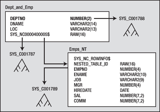
The code created two real tables. The table we asked to have is there, but it has an extra hidden column (we'll have one extra hidden column by default for each nested table column in a table). It also created a unique constraint on this hidden column. Oracle created the nested table, EMPS_NT, for us. This table has two hidden columns, one of which, SYS_NC_ROWINFO$, is not really a column but a virtual column that returns all of the scalar elements as an object. The other is the foreign key called NESTED_TABLE_ID, which can be joined back to the parent table. Notice the lack of an index on this column. Finally, Oracle added an index on the DEPTNO column in the DEPT_AND_EMP table to enforce the primary key. So, we asked for a table and got a lot more than we bargained for. If you look at it, it is a lot like what you might create for a parent/child relationship, but you would have used the existing primary key on DEPTNO as the foreign key in EMPS_NT instead of generating a surrogate RAW(16) key.

If we look at the DBMS_METADATA.GET_DDL dump of our nested table example, we see the following:

ops$tkyte%ORA11GR2> begin
  2     dbms_metadata.set_transform_param
  3     ( DBMS_METADATA.SESSION_TRANSFORM, 'STORAGE', false );
  4  end;
  5  /
PL/SQL procedure successfully completed.

ops$tkyte%ORA11GR2> select dbms_metadata.get_ddl( 'TABLE', 'DEPT_AND_EMP' ) from dual;

DBMS_METADATA.GET_DDL('TABLE','DEPT_AND_EMP')
-------------------------------------------------------------------------------

  CREATE TABLE "OPS$TKYTE"."DEPT_AND_EMP"
   (    "DEPTNO" NUMBER(2,0),
        "DNAME" VARCHAR2(14),
        "LOC" VARCHAR2(13),
        "EMPS" "OPS$TKYTE"."EMP_TAB_TYPE" ,
         PRIMARY KEY ("DEPTNO")

USING INDEX PCTFREE 10 INITRANS 2 MAXTRANS 255
  TABLESPACE "USERS"  ENABLE
   ) SEGMENT CREATION IMMEDIATE
  PCTFREE 10 PCTUSED 40 INITRANS 1 MAXTRANS 255 NOCOMPRESS LOGGING
  TABLESPACE "USERS"
 NESTED TABLE "EMPS" STORE AS "EMPS_NT"
 (( CONSTRAINT "EMPS_EMPNO_UNIQUE" UNIQUE ("EMPNO")
  USING INDEX PCTFREE 10 INITRANS 2 MAXTRANS 255 COMPUTE STATISTICS
  TABLESPACE "USERS"  ENABLE)
PCTFREE 10 PCTUSED 40 INITRANS 1 MAXTRANS 255 LOGGING
  TABLESPACE "USERS" ) RETURN AS VALUE

The only new thing here so far is the RETURN AS VALUE clause. It is used to describe how the nested table is returned to a client application. By default, Oracle will return the nested table by value to the client; the actual data will be transmitted with each row. This can also be set to RETURN AS LOCATOR, meaning the client will get a pointer to the data, not the data itself. If—and only if—the client dereferences this pointer will the data be transmitted to it. So, if you believe the client will typically not look at the rows of a nested table for each parent row, you can return a locator instead of the values, saving on the network round-trips. For example, if you have a client application that displays the lists of departments and when the user double-clicks a department it shows the employee information, you may consider using the locator. This is because the details are usually not looked at—that is the exception, not the rule.

So, what else can we do with the nested table? First, the NESTED_TABLE_ID column must be indexed. Since we always access the nested table from the parent to the child, we really need that index. We can index that column using CREATE INDEX, but a better solution is to use an IOT to store the nested table. The nested table is another perfect example of what an IOT is excellent for. It will physically store the child rows co-located by NESTED_TABLE_ID (so retrieving the table is done with less physical I/O). It will remove the need for the redundant index on the RAW(16) column. Going one step further, since the NESTED_TABLE_ID will be the leading column in the IOT's primary key, we should also incorporate index key compression to suppress the redundant NESTED_TABLE_IDs that would be there otherwise. In addition, we can incorporate our UNIQUE and NOT NULL constraint on the EMPNO column into the CREATE TABLE command. Therefore, if we take the preceding CREATE TABLE statement and modify it slightly

ops$tkyte%ORA11GR2> CREATE TABLE "OPS$TKYTE"."DEPT_AND_EMP"
  2  ("DEPTNO" NUMBER(2, 0),
  3   "DNAME"  VARCHAR2(14),
  4   "LOC"    VARCHAR2(13),
  5  "EMPS" "EMP_TAB_TYPE")
  6  PCTFREE 10 PCTUSED 40 INITRANS 1 MAXTRANS 255 LOGGING
  7  STORAGE(INITIAL 131072 NEXT 131072
  8          MINEXTENTS 1 MAXEXTENTS 4096
  9          PCTINCREASE 0 FREELISTS 1 FREELIST GROUPS 1
 10          BUFFER_POOL DEFAULT)
 11  TABLESPACE "USERS"
 12  NESTED TABLE "EMPS"
 13     STORE AS "EMPS_NT"
 14     ( (empno NOT NULL, unique (empno), primary key(nested_table_id,empno))
 15       organization index compress 1 )
 16     RETURN AS VALUE
 17  /
Table created.

we now get the following set of objects. Instead of having a conventional table EMPS_NT, we have an IOT EMPS_NT as signified by the index structure overlaid on the table in Figure 10-12.

Figure 10-12. Nested table implemented as an IOT

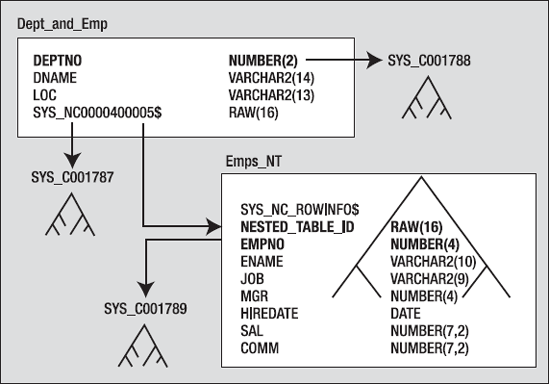
Where the EMPS_NT is an IOT using compression, it should take less storage than the original default nested table and it has the index we badly need.

Temporary tables are used to hold intermediate resultsets for the duration of either a transaction or a session. The data held in a temporary table is only ever visible to the current session—no other session will see any other session's data, even if the current session COMMITs the data. Multiuser concurrency is not an issue with regard to temporary tables either, as one session can never block another session by using a temporary table. Even if we "lock" the temporary table, it will not prevent other sessions from using their temporary table. As we observed in Chapter 9, temporary tables generate significantly less redo than regular tables would. However, since they must generate undo information for the data they contain, they will generate some amount of redo. UPDATEs and DELETEs will generate the largest amount; INSERTs and SELECTs the least amount.

Temporary tables will allocate storage from the currently logged-in user's temporary tablespace, or if they are accessed from a definer rights procedure, the temporary tablespace of the owner of that procedure will be used. A global temporary table is really just a template for the table itself. The act of creating a temporary table involves no storage allocation; no INITIAL extent is allocated, as it would be for a regular table. Rather, at runtime when a session first puts data into the temporary table, a temporary segment for that session will be created. Since each session gets its own temporary segment (not just an extent of an existing segment), every user might be allocating space for her temporary table in different tablespaces. USER1 might have his temporary tablespace set to TEMP1, so his temporary tables will be allocated from this space. USER2 might have TEMP2 as her temporary tablespace, and her temporary tables will be allocated there.

Oracle's temporary tables are similar to temporary tables in other relational databases, with the main exception being that they are statically defined. You create them once per database, not once per stored procedure in the database. They always exist—they will be in the data dictionary as objects, but they will always appear empty until your session puts data into them. The fact that they are statically defined allows you to create views that reference temporary tables, to create stored procedures that use static SQL to reference them, and so on.

Temporary tables may be session based (data survives in the table across commits but not a disconnect/reconnect). They may also be transaction based (data disappears after a commit). Here is an example showing the behavior of both. I used the SCOTT.EMP table as a template:

ops$tkyte@ORA11GR2> create global temporary table temp_table_session
  2  on commit preserve rows
  3  as
  4  select * from scott.emp where 1=0
  5  /
Table created.

The ON COMMIT PRESERVE ROWS clause makes this a session-based temporary table. Rows will stay in this table until my session disconnects or I physically remove them via a DELETE or TRUNCATE. Only my session can see these rows; no other session will ever see my rows, even after I COMMIT.

ops$tkyte@ORA11GR2> create global temporary table temp_table_transaction
  2  on commit delete rows
  3  as
  4  select * from scott.emp where 1=0
  5  /
Table created.

The ON COMMIT DELETE ROWS makes this a transaction-based temporary table. When my session commits, the rows disappear. The rows will disappear by simply giving back the temporary extents allocated to my table—there is no overhead involved in the automatic clearing of temporary tables.

Now, let's look at the differences between the two types:

ops$tkyte@ORA11GR2> insert into temp_table_session select * from scott.emp;
14 rows created.

ops$tkyte@ORA11GR2> insert into temp_table_transaction select * from scott.emp;
14 rows created.

We've just put 14 rows into each TEMP table, and this shows we can see them:

ops$tkyte@ORA11GR2> select session_cnt, transaction_cnt
  2    from ( select count(*) session_cnt from temp_table_session ),
  3         ( select count(*) transaction_cnt from temp_table_transaction );

SESSION_CNT TRANSACTION_CNT
----------- ---------------
         14              14

ops$tkyte@ORA11GR2> commit;

Since we've committed, we'll see the session-based rows but not the transaction-based rows:

ops$tkyte@ORA11GR2> select session_cnt, transaction_cnt
  2    from ( select count(*) session_cnt from temp_table_session ),
  3         ( select count(*) transaction_cnt from temp_table_transaction );

SESSION_CNT TRANSACTION_CNT
----------- ---------------
         14               0

ops$tkyte@ORA11GR2>
ops$tkyte@ORA11GR2> disconnect
Disconnected from Oracle Database 11g Enterprise Edition Release 11.2.0.1.0 - Production
With the Partitioning, OLAP, Data Mining and Real Application Testing optionsops$tkyte@ORA11GR2> connect /
Connected.

Since we've started a new session, we'll see no rows in either table:

ops$tkyte@ORA11GR2> select session_cnt, transaction_cnt
  2    from ( select count(*) session_cnt from temp_table_session ),
  3         ( select count(*) transaction_cnt from temp_table_transaction );

SESSION_CNT TRANSACTION_CNT
----------- ---------------
          0               0

If you have experience of temporary tables in SQL Server and/or Sybase, the major consideration for you is that instead of executing SELECT X, Y, Z INTO #TEMP FROM SOME_TABLE to dynamically create and populate a temporary table, you will

Just to drive home the point, the goal here is not to create tables in your stored procedures at runtime. That is not the proper way to use temporary tables in Oracle. DDL is an expensive operation; you want to avoid doing that at runtime. The temporary tables for an application should be created during the application installation—never at runtime. The pitfalls you will encounter if you attempt to dynamically create the global temporary tables (or just tables in general) at runtime in PL/SQL will be:

In short, there are no good reasons to create tables in PL/SQL at runtime, only reasons to not ever create tables in PL/SQL at run time.

Temporary tables can have many of the attributes of a permanent table. They may have triggers, check constraints, indexes, and so on. Features of permanent tables that they do not support include the following:

One of the drawbacks of a temporary table in any database is the fact that the optimizer has no real statistics on it normally. When using the cost-based optimizer (CBO), valid statistics are vital to the optimizer's success (or failure). In the absence of statistics, the optimizer will make guesses as to the distribution of data, the amount of data, and the selectivity of an index. When these guesses are wrong, the query plans generated for queries that make heavy use of temporary tables could be less than optimal. In many cases, the correct solution is to not use a temporary table at all, but rather to use an INLINE VIEW (for an example of an INLINE VIEW, refer to the last SELECT just run—it has two of them) in its place. In this fashion, Oracle will have access to all of the relevant statistics for a table and can come up with an optimal plan.

I find many times people use temporary tables because they learned in other databases that joining too many tables in a single query is a bad thing. This is a practice that must be unlearned for Oracle development. Rather than trying to outsmart the optimizer and breaking what should be a single query into three or four queries that store their subresults into temporary tables and then combining the temporary tables, you should just code a single query that answers the original question. Referencing many tables in a single query is OK; the temporary table crutch is not needed in Oracle for this purpose.

In other cases, however, the use of a temporary table in a process is the correct approach. For example, I once wrote a Palm sync application to synchronize the date book on a Palm Pilot with calendar information stored in Oracle. The Palm gives me a list of all records that have been modified since the last hot synchronization. I must take these records and compare them against the live data in the database, update the database records, and then generate a list of changes to be applied to the Palm. This is a perfect example of when a temporary table is very useful. I used a temporary table to store the changes from the Palm in the database. I then ran a stored procedure that bumps the Palm-generated changes against the live (and very large) permanent tables to discover what changes need to be made to the Oracle data, and then to find the changes that need to come from Oracle back down to the Palm. I have to make a couple of passes on this data. First, I find all records that were modified only on the Palm and make the corresponding changes in Oracle. I next find all records that were modified on both the Palm and my database since the last synchronization and rectify them. Then I find all records that were modified only on the database and place their changes into the temporary table. Lastly, the Palm sync application pulls the changes from the temporary table and applies them to the Palm device itself. Upon disconnection, the temporary data goes away.

The issue I encountered, however, is that because the permanent tables were analyzed, the CBO was being used. The temporary table had no statistics on it (you can analyze the temporary table but no statistics are gathered), and the CBO would guess many things about it. I, as the developer, knew the average number of rows I might expect, the distribution of the data, the selectivity of the indexes, and so on. I needed a way to inform the optimizer of these better guesses. There are three ways to give the optimizer statistics on the global temporary tables. One is via dynamic sampling (new in Oracle9i Release 2 and above) and the other is the DBMS_STATS package, which has two ways to accomplish this. First, let's look at dynamic sampling.

Dynamic sampling is the optimizer's ability, when hard parsing a query, to scan segments in the database (sample them) to collect statistics useful in optimizing that particular query. It is akin to doing a miniature gather statistics command during a hard parse. In Oracle 10g and above, dynamic sampling will work out of the box, because the default setting has been increased from 1 to 2; at level 2, the optimizer will dynamically sample any unanalyzed object referenced in a query processed by the optimizer prior to evaluating the query plan. In 9i Release 2, the setting of 1 would cause dynamic sampling to be used much less often. We can use an ALTER SESSION|SYSTEM command in Oracle9i Release 2 to make it behave the way Oracle 10g does by default, or we can use the dynamic sampling hint as follows:

ops$tkyte@ORA9IR2> create global temporary table gtt
  2  as
  3  select * from scott.emp where 1=0;
Table created.

ops$tkyte@ORA9IR2> insert into gtt select * from scott.emp;
14 rows created.

ops$tkyte@ORA9IR2> set autotrace traceonly explain
ops$tkyte@ORA9IR2> select /*+ first_rows */ * from gtt;

Execution Plan
----------------------------------------------------------
   0      SELECT STATEMENT Optimizer=HINT: FIRST_ROWS (Cost=17 Card=8168 Bytes...
   1    0   TABLE ACCESS (FULL) OF 'GTT' (Cost=17 Card=8168 Bytes=710616)

ops$tkyte@ORA9IR2> select /*+ first_rows dynamic_sampling(gtt 2) */ * from gtt;

Execution Plan
----------------------------------------------------------
   0      SELECT STATEMENT Optimizer=HINT: FIRST_ROWS (Cost=17 Card=14 Bytes=1218)
   1    0   TABLE ACCESS (FULL) OF 'GTT' (Cost=17 Card=14 Bytes=1218)

ops$tkyte@ORA9IR2> set autotrace off

Here, we set the dynamic sampling to level 2 for the table GTT in this query. Left to itself, the optimizer guessed 8,168 rows would be returned from the table GTT.

Using dynamic sampling, the estimated cardinality will be much closer to reality (which leads to better query plans overall). Using the level 2 setting, the optimizer quickly scans the table to come up with more-realistic estimates of the true size of this table. In Oracle 10g, we should find this to be less of a problem, because the defaults will cause dynamic sampling to take place:

ops$tkyte@ORA11GR2> create global temporary table gtt
  2  as
  3  select * from scott.emp where 1=0;
Table created.

ops$tkyte@ORA11GR2> insert into gtt select * from scott.emp;
14 rows created.

ops$tkyte@ORA11GR2> set autotrace traceonly explain
ops$tkyte@ORA11GR2> select * from gtt;

Execution Plan
----------------------------------------------------------
   0      SELECT STATEMENT Optimizer=ALL_ROWS (Cost=2 Card=14 Bytes=1218)
   1    0   TABLE ACCESS (FULL) OF 'GTT' (TABLE (TEMP)) (Cost=2 Card=14 Bytes=1218)

ops$tkyte@ORA11GR2> set autotrace off

We get the right cardinality without having to ask for it. Dynamic sampling does not come free, however—there is a cost associated with having to perform it at query parse time. If we gathered appropriate representative statistics ahead of time, we could avoid this at hard parse time. That leads us into DBMS_STATS.

There are three methods to use DBMS_STATS to gather representative statistics. The first way is to use DBMS_STATS with the GATHER_SCHEMA_STATS, or GATHER_DATABASE_STATS call. These procedures allow you to pass in a parameter, GATHER_TEMP, which is a Boolean and defaults to FALSE. When set to TRUE, any ON COMMIT PRESERVE ROWS global temporary table will have statistics gathered and stored (this technique will not work on ON COMMIT DELETE ROWS tables). Consider the following (note that this was done in an empty schema; the only objects are those you see created):

ops$tkyte@ORA11GR2> create table emp as select * from scott.emp;
Table created.

ops$tkyte@ORA11GR2> create global temporary table gtt1 ( x number )
  2  on commit preserve rows;
Table created.

ops$tkyte@ORA11GR2> create global temporary table gtt2 ( x number )
  2  on commit delete rows;
Table created.

ops$tkyte@ORA11GR2> insert into gtt1 select user_id from all_users;
38 rows created.

ops$tkyte@ORA11GR2> insert into gtt2 select user_id from all_users;
38 rows created.

ops$tkyte@ORA11GR2> exec dbms_stats.gather_schema_stats( user );
PL/SQL procedure successfully completed.

ops$tkyte@ORA11GR2> select table_name, last_analyzed, num_rows from user_tables;

TABLE_NAME                     LAST_ANAL   NUM_ROWS
------------------------------ --------- ----------
EMP                            01-MAY-10         14
GTT1
GTT2

As you can see, only the EMP table was analyzed in this case; the two global temporary tables were ignored. We can change that behavior by calling GATHER_SCHEMA_STATS with GATHER_TEMP => TRUE:

ops$tkyte@ORA11GR2> insert into gtt2 select user_id from all_users;
38 rows created.

ops$tkyte@ORA11GR2> exec dbms_stats.gather_schema_stats( user, gather_temp=>TRUE );
PL/SQL procedure successfully completed.

ops$tkyte@ORA11GR2> select table_name, last_analyzed, num_rows from user_tables;

TABLE_NAME                     LAST_ANAL   NUM_ROWS
------------------------------ --------- ----------
EMP                            01-MAY-10         14
GTT1                           01-MAY-10         38
GTT2                           01-MAY-10          0

Notice that the ON COMMIT PRESERVE rows table has accurate statistics, but the ON COMMIT DELETE ROWS does not. DBMS_STATS commits and that wipes out any information in that table. Do note, however, that GTT2 does now have statistics, which in itself is a bad thing, because the statistics are very much incorrect! It is doubtful the table will have 0 rows in it at runtime. So, if you use this approach, be aware of two things:

The second technique that works with ON COMMIT PRESERVE ROWS global temporary tables is to use GATHER_TABLE_STATS directly on the table. You would populate the global temporary table as we just did, and then execute GATHER_TABLE_STATS on that global temporary table. Note that just as before, this does not work for ON COMMIT DELETE ROWS global temporary tables, as the same issues as just described would come into play.

The last technique using DBMS_STATS uses a manual process to populate the data dictionary with representative statistics for our temporary tables. For example, if on average the number of rows in the temporary table will be 500, the average row size will be 100 bytes, and the number of blocks will be 7, we could simply use the following:

ops$tkyte@ORA11GR2> create global temporary table t ( x int, y varchar2(100) );
Table created.

ops$tkyte@ORA11GR2> begin
  2     dbms_stats.set_table_stats( ownname => USER,
  3                                 tabname => 'T',
  4                                 numrows => 500,
  5                                 numblks => 7,
  6                                 avgrlen => 100 );
  7  end;
  8  /
PL/SQL procedure successfully completed.

ops$tkyte@ORA11GR2> select table_name, num_rows, blocks, avg_row_len
  2               from user_tables
  3              where table_name = 'T';

TABLE_NAME                       NUM_ROWS     BLOCKS AVG_ROW_LEN
------------------------------ ---------- ---------- -----------
T                                     500          7         100

Now, the optimizer won't use its best guess—it will use our best guess for this information.

We have already seen a partial example of an object table with nested tables. An object table is a table that is created based on a TYPE, not as a collection of columns. Normally, a CREATE TABLE statement would look like this:

create table t ( x int, y date, z varchar2(25) );

An object table creation statement looks more like this:

create table t of Some_Type;

The attributes (columns) of T are derived from the definition of SOME_TYPE. Let's quickly look at an example involving a couple of types, and then review the resulting data structures:

ops$tkyte@ORA11GR2> create or replace type address_type
  2  as object
  3  ( city    varchar2(30),
  4    street  varchar2(30),
  5    state   varchar2(2),
  6    zip     number
  7  )
  8  /
Type created.

ops$tkyte@ORA11GR2> create or replace type person_type
  2  as object
  3  ( name             varchar2(30),
  4    dob              date,
  5    home_address     address_type,
  6    work_address     address_type
  7  )
  8  /
Type created.

ops$tkyte@ORA11GR2> create table people of person_type
  2  /
Table created.

ops$tkyte@ORA11GR2> desc people
 Name                                     Null?    Type
 ---------------------------------------- -------- ----------------------------
 NAME                                              VARCHAR2(30)
 DOB                                               DATE
 HOME_ADDRESS                                      ADDRESS_TYPE
 WORK_ADDRESS                                      ADDRESS_TYPE

In a nutshell, that's all there is to it. We create some type definitions, and then we can create tables of that type. The table appears to have four columns representing the four attributes of the PERSON_TYPE we created. We are at the point where we can now perform DML on the object table to create and query data:

ops$tkyte@ORA11GR2> insert into people values ( 'Tom', '15-mar-1965',
  2  address_type( 'Reston', '123 Main Street', 'Va', '45678' ),
  3  address_type( 'Redwood', '1 Oracle Way', 'Ca', '23456' ) );
1 row created.

ops$tkyte%ORA11GR2> select name, dob, p.home_address Home, p.work_address work
  2    from people p;

NAME DOB       HOME(CITY, STREET, STA WORK(CITY, STREET, STAT
---- --------- ---------------------- -----------------------
Tom  15-MAR-65 ADDRESS_TYPE('Reston', ADDRESS_TYPE('Redwood',
               '123 Main Street',     '1 Oracle Way', 'Ca',
               'Va', 45678)           23456)


ops$tkyte@ORA11GR2> select name, p.home_address.city from people p;

NAME  HOME_ADDRESS.CITY
----- ------------------------------
Tom   Reston

We're starting to see some of the object syntax necessary to deal with object types. For example, in the INSERT statement we had to wrap the HOME_ADDRESS and WORK_ADDRESS with a CAST. We cast the scalar values to be of an ADDRESS_TYPE. Another way of saying this is that we create an ADDRESS_TYPE instance for that row by using the default constructor for the ADDRESS_TYPE object.

Now, as far as the external face of the table is concerned, there are four columns in our table. By now, after seeing the hidden magic that took place for the nested tables, we can probably guess that there is something else going on. Oracle stores all object relational data in plain old relational tables—at the end of the day, it is all in rows and columns. If we dig into the real data dictionary, we can see what this table really looks like:

ops$tkyte@ORA11GR2> select name, segcollength
  2    from sys.col$
  3   where obj# = ( select object_id
  4                    from user_objects
  5                   where object_name = 'PEOPLE' )
  6  /

NAME                      SEGCOLLENGTH
------------------------- ------------
SYS_NC_OID$                         16
SYS_NC_ROWINFO$                      1
NAME                                30
DOB                                  7
HOME_ADDRESS                         1
SYS_NC00006$                        30
SYS_NC00007$                        30
SYS_NC00008$                         2
SYS_NC00009$                        22
WORK_ADDRESS                         1
SYS_NC00011$                        30
SYS_NC00012$                        30
SYS_NC00013$                         2
SYS_NC00014$                        22
 14 rows selected.

This looks quite different from what DESCRIBE tells us. Apparently, there are 14 columns in this table, not 4. In this case, they are:

So, just like with the nested table, there is a lot going on here. A pseudo primary key of 16 bytes was added, there are virtual columns, and an index created for us. We can change the default behavior with regard to the value of the object identifier assigned to an object, as we'll see in a moment. First, let's look at the full verbose SQL that would generate our table for us. This was generated using EXP/IMP since I wanted to easily see the dependent objects, including all of the SQL needed to re-create this particular object instance. This was achieved via the following:

$ exp userid=/ tables=people rows=n
Export: Release 11.2.0.1.0 - Production on Thu Mar 18 10:17:52 2010
Copyright (c) 1982, 2009, Oracle and/or its affiliates.  All rights reserved.

Connected to: Oracle Database 11g Enterprise Edition Release 11.2.0.1.0 - Production
With the Partitioning, OLAP, Data Mining and Real Application Testing options
Export done in US7ASCII character set and AL16UTF16 NCHAR character set
server uses WE8MSWIN1252 character set (possible charset conversion)
Note: table data (rows) will not be exported

About to export specified tables via Conventional Path ...
. . exporting table                         PEOPLE
Export terminated successfully without warnings.

$ imp userid=/ indexfile=people.sql full=y
Import: Release 11.2.0.1.0 - Production on Thu Mar 18 10:18:10 2010
Copyright (c) 1982, 2009, Oracle and/or its affiliates.  All rights reserved.

Connected to: Oracle Database 11g Enterprise Edition Release 11.2.0.1.0 - Production
With the Partitioning, OLAP, Data Mining and Real Application Testing options

Export file created by EXPORT:V11.02.00 via conventional path
import done in US7ASCII character set and AL16UTF16 NCHAR character set
import server uses WE8MSWIN1252 character set (possible charset conversion)
Import terminated successfully without warnings.

Review of the people.sql file that results would show this:

CREATE TABLE "OPS$TKYTE"."PEOPLE"
OF "PERSON_TYPE" OID '82149DEE11C135AAE040A8C0FC011326'
OIDINDEX (PCTFREE 10 INITRANS 2 MAXTRANS 255
          STORAGE(INITIAL 65536 NEXT 1048576
                  MINEXTENTS 1 FREELISTS 1
                  FREELIST GROUPS 1
                  BUFFER_POOL DEFAULT)
  TABLESPACE "USERS")
  PCTFREE 10 PCTUSED 40
  INITRANS 1 MAXTRANS 255
  STORAGE(INITIAL 65536 NEXT 1048576
          MINEXTENTS 1 FREELISTS 1
          FREELIST GROUPS 1
          BUFFER_POOL DEFAULT)
 TABLESPACE "USERS" LOGGING NOCOMPRESS ;

ALTER TABLE "OPS$TKYTE"."PEOPLE"
MODIFY ("SYS_NC_OID$" DEFAULT SYS_OP_GUID()) ;

This gives us a little more insight into what is actually taking place here. We see the OIDINDEX clause clearly now, and we see a reference to the SYS_NC_OID$ column. This is the hidden primary key of the table. The function SYS_OP_GUID is the same as the function SYS_GUID. They both return a globally unique identifier that is a 16-byte RAW field.

The OID '<big hex number>' syntax is not documented in the Oracle documentation. All this is doing is ensuring that during an EXP and subsequent IMP, the underlying type PERSON_TYPE is, in fact, the same type. This will prevent an error that would occur if we performed the following steps:

Obviously, this export cannot be imported into the new structure—it will not fit. This check prevents that from occurring.

If you remember, I mentioned that we can change the behavior of the object identifier assigned to an object instance. Instead of having the system generate a pseudo primary key for us, we can use the natural key of an object. At first, this might appear self-defeating—the SYS_NC_OID$ column will still appear in the table definition in SYS.COL$ and, in fact, it will appear to consume massive amounts of storage as compared to the system-generated column. Once again, however, there is magic at work here. The SYS_NC_OID$ column for an object table that is based on a primary key and not system generated is a virtual column and consumes no real storage on disk.

Here is an example that shows what happens in the data dictionary and demonstrates that there is no physical storage consumed for the SYS_NC_OID$ column. We'll start with an analysis of the system-generated OID table:

ops$tkyte@ORA11GR2> create table people of person_type
  2  /
Table created.

ops$tkyte@ORA11GR2> select name, type#, segcollength
  2    from sys.col$
  3   where obj# = ( select object_id
  4                    from user_objects
  5                   where object_name = 'PEOPLE' )
  6     and name like 'SYS\_NC\_%' escape ''
  7  /

NAME                           TYPE# SEGCOLLENGTH
------------------------- ---------- ------------
SYS_NC_OID$                       23           16
SYS_NC_ROWINFO$                  121            1

ops$tkyte@ORA11GR2> insert into people(name)
  2  select rownum from all_objects;
48217 rows created.

ops$tkyte@ORA11GR2> exec dbms_stats.gather_table_stats( user, 'PEOPLE' );
PL/SQL procedure successfully completed.

ops$tkyte@ORA11GR2> select table_name, avg_row_len from user_object_tables;

TABLE_NAME                     AVG_ROW_LEN
------------------------------ -----------
PEOPLE                                  23

We see here that the average row length is 23 bytes: 16 bytes for the SYS_NC_OID$ column and 7 bytes for the NAME column. Now, let's do the same thing, but use a primary key on the NAME column as the object identifier:

ops$tkyte@ORA11GR2> CREATE TABLE "PEOPLE"
  2  OF "PERSON_TYPE"
  3  ( constraint people_pk primary key(name) )
  4  object identifier is PRIMARY KEY
  5  /
Table created.

ops$tkyte@ORA11GR2> select name, type#, segcollength
  2    from sys.col$
  3   where obj# = ( select object_id
  4                    from user_objects
  5                   where object_name = 'PEOPLE' )
  6     and name like 'SYS\_NC\_%' escape ''
  7  /

NAME                                TYPE# SEGCOLLENGTH
------------------------------ ---------- ------------
SYS_NC_OID$                            23           81
SYS_NC_ROWINFO$                       121            1

According to this, instead of a small 16-byte column, we have a large 81-byte column! In reality, there is no data stored in there. It will be null. The system will generate a unique ID based on the object table, its underlying type, and the value in the row itself. We can see this in the following:

ops$tkyte@ORA11GR2> insert into people (name)
  2  values ( 'Hello World!' );
1 row created.

ops$tkyte@ORA11GR2> select sys_nc_oid$ from people p;

SYS_NC_OID$
-------------------------------------------------------------------------------
F610733A48F865F9E030007F0100149A00000017260100010001002900000000000C07001E01000
02A00078401FE000000140C 48656C6C6F20576F726C642100000000000000000000000000000000
0000

ops$tkyte@ORA11GR2> select utl_raw.cast_to_raw( 'Hello World!' ) data
  2  from dual;

DATA
-------------------------------------------------------------------------------
48656C6C6F20576F726C6421

ops$tkyte@ORA11GR2> select utl_raw.cast_to_varchar2(sys_nc_oid$) data
  2  from people;

DATA
-------------------------------------------------------------------------------
<garbage bits and bytes..>Hello World!

If we select out the SYS_NC_OID$ column and inspect the HEX dump of the string we inserted, we see that the row data itself is embedded in the object ID. Converting the object ID into a VARCHAR2, we can just confirm that visually. Does that mean our data is stored twice with a lot of overhead with it? No, it is not—it is just factored into that magic thing that is the SYS_NC_OID$ column upon retrieval. Oracle synthesizes the data upon selecting from the table.

Now for an opinion. The object relational components (nested tables and object tables) are primarily what I call syntactic sugar. They are always translated into good old relational rows and columns. I prefer not to use them as physical storage mechanisms personally. There are too many bits of magic happening—side effects that are not clear. You get hidden columns, extra indexes, surprise pseudo columns, and so on. This does not mean that the object-relational components are a waste of time. On the contrary, I use them in PL/SQL constantly. I use them with object views. I can achieve the benefits of a nested table construct (less data returned over the network for a master/detail relationship, conceptually easier to work with, and so on) without any of the physical storage concerns. That is because I can use object views to synthesize my objects from my relational data. This solves most of my concerns with object tables/nested tables in that the physical storage is dictated by me, the join conditions are set up by me, and the tables are available as relational tables (which is what many third-party tools and applications will demand) naturally. The people who require an object view of relational data can have it, and the people who need the relational view can have it. Since object tables are really relational tables in disguise, we are doing the same thing Oracle does for us behind the scenes, only we can do it more efficiently, since we don't have to do it generically as they do. For example, using the types defined earlier, I could just as easily use the following:

ops$tkyte@ORA11GR2> create table people_tab
  2  (  name        varchar2(30) primary key,
  3     dob         date,
  4     home_city   varchar2(30),
  5     home_street varchar2(30),
  6     home_state  varchar2(2),
  7     home_zip    number,
  8     work_city   varchar2(30),
  9     work_street varchar2(30),
 10     work_state  varchar2(2),
 11     work_zip    number
 12  )
 13  /
Table created.

ops$tkyte@ORA11GR2> create view people of person_type
  2  with object identifier (name)
  3  as
  4  select name, dob,
  5    address_type(home_city,home_street,home_state,home_zip) home_adress,
  6   address_type(work_city,work_street,work_state,work_zip) work_adress
  7    from people_tab
  8  /
View created.

ops$tkyte@ORA11GR2> insert into people values ( 'Tom', '15-mar-1965',
  2  address_type( 'Reston', '123 Main Street', 'Va', '45678' ),
  3  address_type( 'Redwood', '1 Oracle Way', 'Ca', '23456' ) );
1 row created.

However, I achieve very much the same effect, I know exactly what is stored, how it is stored, and where it is stored. For more complex objects, we may have to code INSTEAD OF triggers on the object views to allow for modifications through the view.

Hopefully, after reading this chapter you have come to the conclusion that not all tables are created equal. Oracle provides a rich variety of table types that you can exploit. In this chapter, we have covered many of the salient aspects of tables in general and explored the many different table types Oracle provides for us to use.

We began by looking at some terminology and storage parameters associated with tables. We looked at the usefulness of FREELISTs in a multiuser environment where a table is frequently inserted/updated by many people simultaneously, and how the use of ASSM tablespaces could make it so we don't even have to think about that. We investigated the meaning of PCTFREE and PCTUSED, and we developed some guidelines for setting them correctly.

Then we got into the different types of tables, starting with the common heap. The heap organized table is by far the most commonly used table in most Oracle applications, and it is the default table type. We moved on to examine index organized tables, which provide us with the ability to store our table data in an index structure instead of a heap table. We saw how these are applicable for various uses, such as lookup tables and inverted lists, where a heap table would just be a redundant copy of the data. Later, we saw how IOTs can really be useful when mixed with other table types, specifically the nested table type.

We looked at cluster objects, of which Oracle has three kinds: index, hash, and sorted hash. The goals of the cluster are twofold:

These features allow us to access related data very quickly with minimal physical I/O. We observed the main differences between index clusters and hash clusters, and we discussed when each would (and would not) be appropriate.

Next, we covered nested tables. We reviewed the syntax, semantics, and usage of nested tables. We saw how they are, in fact, a system-generated and maintained parent/child pair of tables, and we discovered how Oracle physically does this for us. We looked at using different table types for nested tables, which by default use a heap-based table. We found that there will probably never be a reason not to use an IOT instead of a heap table for nested tables.

Then we looked into the ins and outs of temporary tables, including how to create them, where they get their storage from, and the fact that they introduce no concurrency-related issues at runtime. We explored the differences between session-level and transaction-level temporary tables, and we discussed the appropriate method for using temporary tables in an Oracle database.

This chapter finished with a look into the workings of object tables. As with nested tables, we discovered there is a lot going on under the covers with object tables in Oracle. We discussed how object views on top of relational tables can give us the functionality of an object table, while at the same time giving us easy access to the underlying relational data.