![]()
Retrieval: Some Advanced Features
This is the fourth chapter in a series about retrieval features of SQL. It is a logical continuation of Chapters 4, 5, and 8.
First, in Section 9.1, we revisit subqueries, beginning with an introduction to the three operators ANY, ALL, and EXISTS. These operators allow you to create a special relationship between main queries and subqueries, as opposed to using the IN operator or standard comparison operators. You will also learn about correlated subqueries, which are subqueries where some subquery clauses refer to column expressions in the main query.
In Sections 9.2 and 9.3, we will look at subqueries in query components other than the WHERE clause: namely, the SELECT and the FROM clauses. In Section 9.4 we will discuss the WITH clause, also referred to as subquery factoring, which allows you to define one or more subqueries in the beginning of your SQL statement commands, and then to reference them by name in the remainder of your SQL statement command.
We continue with hierarchical queries in Section 9.5. Relational tables are essentially flat structures, but they can represent hierarchical data structures; for example, by using foreign key constraints referring to the primary key of the same table. The MGR column of the EMPLOYEES table is a classic example of such a hierarchical relationship (a foreign key is defined from the MGR column to the EMPLOYEE_ID primary key column of the EMPLOYEES table). Oracle SQL supports explicit syntax to simplify retrieval of hierarchical data structures.
The next subject we investigate is analytic functions (Section 9.6). Within the context of a single row (or tuple variable), you can reference data in other rows and use it for comparisons and calculations. Comparatively, Section 9.7 illustrates the row limiting clause you can employ to limit the rows returned by a query and to use simpler syntax that provides you with the ability to page through an ordered set.
Finally, Section 9.8 discusses a helpful Oracle SQL feature allowing you to travel back in time: flashback queries.
9.1 Subqueries Continued
Chapter 4 discussed various examples of subqueries, using the IN operator or standard logical comparison operators. As a refresher, let’s start with two standard subquery examples.
The subquery in Listing 9-1 displays all 13 registrations we have for build courses; that is, for course category 'BLD'.
Listing 9-1. Subquery Using the IN Operator
select r.attendee, r.course, r.begindate
from   registrations r
where  r.course in (select c.code
                   from   courses c
                   where  c.category='BLD'),

ATTENDEE COURSE BEGINDATE
-------- ------ -----------
    7499 JAV    13-DEC-1999
    7566 JAV    01-FEB-2000
    7698 JAV    01-FEB-2000
    7788 JAV    13-DEC-1999
    7839 JAV    13-DEC-1999
    7876 JAV    13-DEC-1999
    7788 JAV    01-FEB-2000
    7782 JAV    13-DEC-1999
    7499 PLS    11-SEP-2000
    7876 PLS    11-SEP-2000
    7566 PLS    11-SEP-2000
    7499 XML    03-FEB-2000
    7900 XML    03-FEB-2000
Listing 9-2 shows how you can retrieve all employees who are younger than colleague 7566.
Listing 9-2. Single-Row Subquery Using a Comparison Operator
select e.empno, e.ename, e.init, e.bdate
from   employees e
where  e.bdate > (select x.bdate
                  from   employees x
                  where  x.empno = 7566);

   EMPNO ENAME    INIT  BDATE
-------- -------- ----- -----------
    7844 TURNER   JJ    28-SEP-1968
    7900 JONES    R     03-DEC-1969
Listing 9-2 shows an example of a single-row subquery. The subquery must return a single row, because the comparison operator (>) in the third line of the outer query would fail otherwise. If subqueries of this type nevertheless return more than a single row, you receive an Oracle error message, as you discovered in Chapter 4 (see Listing 4-38).
The following section continues the discussion of subqueries by explaining the possibilities of the ANY, ALL, and EXISTS operators. You’ll also learn about correlated subqueries.
The ANY and ALL Operators
SQL allows you to combine standard comparison operators (<, >, =, and so on) with subqueries returning any number of rows. You can do that by specifying ANY or ALL between the comparison operator and the subquery. Listing 9-3 illustrates an example of using the ANY operator, showing all employees with a monthly salary that is higher than at least one manager.
Listing 9-3. ANY Operator Example
select e.empno, e.ename, e.job, e.msal
from   employees e
where  e.msal > ANY (select x.msal
                     from   employees x
                     where  x.job = 'MANAGER'),

   EMPNO ENAME    JOB          MSAL
-------- -------- -------- --------
    7839 KING     DIRECTOR     5000
    7788 SCOTT    TRAINER      3000
    7902 FORD     TRAINER      3000
    7566 JONES    MANAGER      2975
    7698 BLAKE    MANAGER      2850
Listing 9-4 shows an example of using the ALL operator, showing the “happy few” with a higher salary than all managers.
Listing 9-4. ALL Operator Example
select e.empno, e.ename, e.job, e.msal
from   employees e
where  e.msal > ALL (select x.msal
                     from   employees x
                     where  x.job = 'MANAGER'),

   EMPNO ENAME    JOB          MSAL
-------- -------- -------- --------
    7788 SCOTT    TRAINER      3000
    7839 KING     DIRECTOR     5000
    7902 FORD     TRAINER      3000
Defining ANY and ALL
As the examples illustrate, the ANY and ALL operators work as follows:
- ANY: ... means the result is true forat least one valuereturned by the subquery.
- ALL: ... means the result is truefor all valuesreturned by the subquery.
Table 9-1 formulates the definitions of ANY and ALL a bit more formally, using iterated OR and AND constructs. In the table, the symbol, #, represents any standard comparison operator: <, >, =, >=, <=, or <>. Also, V1, V2, V3, and so on represent the values returned by the subquery.
Table 9-1. Definition of ANY and ALL
X # ANY(subquery) |
X # ALL(subquery) |
|---|---|
(X # V1) OR |
(X # V1) AND |
(X # V2) OR |
(X # V2) AND |
(X # V3) OR |
(X # V3) AND |
Rewriting SQL Statements Containing ANY and ALL
In most cases, you can rewrite your SQL statements in such a way that you don’t need the ANY and ALL operators. For example, we could have used a group function in Listing 9-4 to rebuild the subquery into a single-row subquery, as shown in Listing 9-5.
Listing 9-5. Using the MAX Function in the Subquery, Instead of ALL
select e.ename, e.job, e.msal
from   employees e
where  e.msal > (select max(x.msal)
                 from   employees x
                 where  x.job = 'MANAGER'),

ENAME    JOB          MSAL
-------- -------- --------
SCOTT    TRAINER      3000
KING     DIRECTOR     5000
FORD     TRAINER      3000
Note that the following SQL constructs are logically equivalent:
- X = ANY(subquery) <=> X IN (subquery)
- X <> ALL(subquery) <=> X NOT IN (subquery)
Look at the following two rather special cases of ANY and ALL:
- X = ALL(subquery)
- X <> ANY(subquery)
If the subquery returns two or more different values, the first expression is alwaysFALSE, because X can never be equal to two different values at the same time. Likewise, if the subquery returns two or more different values, the second expression is alwaysTRUE, because any X will be different from at least one of those two values from the subquery.
Correlated Subqueries
SQL also supports correlated subqueries. Look at the example in Listing 9-6, and you will find out why these subqueries are referred to as being correlated.
Listing 9-6. Correlated Subquery Example
select e.ename, e.init, e.msal
from   employees e
where  e.msal > (select avg(x.msal)
                 from   employees x
                 where  x.deptno = e.deptno  -- Note the reference to e
                );

ENAME    INIT      MSAL
-------- ----- --------
ALLEN    JAM       1600
JONES    JM        2975
BLAKE    R         2850
SCOTT    SCJ       3000
KING     CC        5000
FORD     MG        3000
You may want to compare this query with Listing 8-30 in the previous chapter, because they are similar. This query displays all employees who earn a higher salary than the average salary of their own department. There is one thing that makes this subquery special: it contains a reference to the tuple variable e (see e.DEPTNO in the fifth line) from the main query. This means that you cannot execute this subquery independently, in isolation, because that would result in an Oracle error message. You must interpret this subquery within the context of a specific row from the main query. The subquery is related to the main query, thus it is referred to as being correlated.
The Oracle DBMS processes the query in Listing 9-6 as follows:
- The tuple variable e ranges over the EMPLOYEES table, thus assuming 14 different values.
- For each row e, the subquery is executed after replacing e.DEPTNO with the literal department value of row e.
![]() Caution Re-executing a subquery for every single row of the main query may have a significant performance impact. The Oracle optimizer will try to produce an efficient execution plan, and there are some smart optimization algorithms for correlated subqueries; nevertheless, it is always a good idea to consider and test performance while writing SQL statements for production systems. With many queries, performance with small data sets (such as you would find in a development database) can be considered to be quite good, but they do not perform well when large, near-production size data sets are queried.
Caution Re-executing a subquery for every single row of the main query may have a significant performance impact. The Oracle optimizer will try to produce an efficient execution plan, and there are some smart optimization algorithms for correlated subqueries; nevertheless, it is always a good idea to consider and test performance while writing SQL statements for production systems. With many queries, performance with small data sets (such as you would find in a development database) can be considered to be quite good, but they do not perform well when large, near-production size data sets are queried.
In mathematics, a distinction is made between free and bound variables. In the subquery of Listing 9-6, x is the free variable and e is bound by the main query.
Let’s look at another example in Listing 9-7. This query returns the fourth youngest employee of the company or, to be more precise, all employees for which there are three younger colleagues. Note that the result isn’t necessarily a set containing a single employee.
Listing 9-7. Another Example of a Correlated Subquery
select e.*
from   employees e
where (select count(*)
       from   employees x
       where  x.bdate > e.bdate) = 3;

 EMPNO ENAME    INIT  JOB         MGR BDATE         MSAL   COMM DEPTNO
------ -------- ----- -------- ------ ----------- ------ ------ ------
  7876 ADAMS    AA    TRAINER    7788 30-DEC-1966   1100            20
You can also formulate these types of queries using analytic functions, as described in Section 9.6 of this chapter.
![]() Note Analytic functions can sometimes help in obtaining certain answers to SQL questions by providing simpler syntax and better performance. However, since an incorrect use of analytic functions can also degrade performance and SQL statement readability, any statement written using an analytic function should be carefully tested and code reviewed.
Note Analytic functions can sometimes help in obtaining certain answers to SQL questions by providing simpler syntax and better performance. However, since an incorrect use of analytic functions can also degrade performance and SQL statement readability, any statement written using an analytic function should be carefully tested and code reviewed.
Correlated subqueries often occur in combination with the EXISTS operator. Again, let’s start with an example. The query in Listing 9-8 returns all course offerings without registrations.
Listing 9-8. Correlated Subquery with EXISTS Operator
select o.*
from   offerings o
where  not exists
      (select r.*
       from   registrations r
       where  r.course    = o.course
       and    r.begindate = o.begindate);

COURSE BEGINDATE    TRAINER LOCATION
------ ----------- -------- --------
ERM    15-JAN-2001
PRO    19-FEB-2001          DALLAS
RSD    24-FEB-2001     7788 CHICAGO
XML    18-SEP-2000          BOSTON
The EXISTS operator is not interested in the actual rows (and column values) resulting from the subquery, if any. This operator checks for only the existence of subquery results. If the subquery returns at least one resulting row, the EXISTS operator evaluates to TRUE. If the subquery returns no rows at all, the result is FALSE.
Subqueries Following an EXISTS Operator
You could say that the EXISTS and NOT EXISTS operators are kind of empty set checkers. This implies that it doesn’t matter which expressions you specify in the SELECT clause of the subquery. For example, you could also have written the query of Listing 9-8 as follows:
select o.*
from   offerings o
where   not exists
       (select 'x'
        from   registrations r ...
![]() Note The ANSI/ISO SQL standard defines * as being an arbitrary literal in this case.
Note The ANSI/ISO SQL standard defines * as being an arbitrary literal in this case.
Subqueries that follow an EXISTS operator are often correlated. Think about this for a moment. If they are uncorrelated, their result is precisely the same for each row from the main query. There are only two possible outcomes: the EXISTS operator results in TRUE for all rows or FALSE for all rows. In other words, EXISTS followed by an uncorrelated subquery becomes an “all or nothing” operator.
![]() Caution A subquery returning a null value is not the same as a subquery returning nothing (that is, the empty set). This will be demonstrated later in this section.
Caution A subquery returning a null value is not the same as a subquery returning nothing (that is, the empty set). This will be demonstrated later in this section.
EXISTS, IN, or JOIN?
See Listing 9-9 for another EXISTS example to finish this section. The query is intended to provide the personal details of all employees who ever taught an SQL course.
Listing 9-9. Another Correlated Subquery with EXISTS Operator
select e.*
from   employees e
where  exists (select o.*
               from   offerings o
               where  o.course = 'SQL'
               and    o.trainer = e.empno);

 EMPNO ENAME    INIT  JOB         MGR BDATE           MSAL   COMM DEPTNO
------ -------- ----- -------- ------ ----------- -------- ------ ------
  7369 SMITH    N     TRAINER    7902 17-DEC-1965      800            20
  7902 FORD     MG    TRAINER    7566 13-FEB-1959     3000            20
This problem can also be solved with an IN operator, as shown in Listing 9-10. The query results are omitted.
Listing 9-10. Alternative Formulation for Listing 9-9
select e.*
from   employees e
where  e.empno in (select o.trainer
                   from   offerings o
                   where  o.course = 'SQL')
You can also use a join to solve the problem, as shown in Listing 9-11. This is probably the most obvious approach, although the choice between writing joins or subqueries is highly subjective. Some people think “bottom up” and prefer subqueries; others think “top down” and prefer to write joins.
Listing 9-11. Another Alternative Formulation for Listing 9-9
select DISTINCT e.*
from   employees e
       join
       offerings o
       on e.empno = o.trainer
where  o.course = 'SQL'
Notice the DISTINCT option in the SELECT clause. Investigate what happens if you remove the DISTINCT option in Listing 9-11. You’ll find that the query result will consist of three rows, instead of two. The query in Listing 9-11 can return multiple instances of the same employee if an employee is teaching more than one offering of the course, “SQL.” Since the query in Listing 9-9 employs a correlated subquery, only two rows are returned. Since an employee is added to the result set once, and only once, it matches a trainer value selected from the correlated subquery.
So far, we have considered only subqueries in the WHERE clause. However, you can use subqueries in other SQL statement components, such as the SELECT and FROM clauses. In the next sections, we will look at subqueries in these other clauses.
NULLs with EXISTS and IN in subquery results often cause problems for people writing SQL for Oracle database systems, especially for those used to writing SQL for other database systems. Not only can NULLs in subquery results cause confusion, but they can lead to incorrect results.
There are several key concepts to keep in mind:
- NULL is not data, but rather a condition of data being unknown.
- Null = Null, NULL != NULL or NULL IN (NULL) always evaluates to UNKNOWN, which is neither TRUE nor FALSE.
- It is not possible to join two rows with NULLs in the join column.
We illustrate our point about the trouble NULLs cause with EXISTS and IN queries with the reports in Listing 9-12. The queries behind the reports show two different ways to generate a list of managers. One approach uses IN; the other uses EXISTS. At face value, either approach works, and there seems to be no difference between them.
Listing 9-12. Selecting All Managers Using IN or EXISTS
select ename
from employees
where empno in (select mgr from employees);

ENAME
--------
JONES
BLAKE
CLARK
SCOTT
KING
FORD

select e1.ename
from employees e1
where exists (select e2.mgr
                 from   employees e2
                 where e1.empno = e2.mgr);

ENAME
--------
JONES
BLAKE
CLARK
SCOTT
KING
FORD
As you see from Listing 9-12, the use of IN or EXISTS are equivalent in terms of results, though the actual operations are different. IN builds a list of values that are used for comparison with EMPNO. EXISTS executes the subquery for each EMPNO and returns TRUE if the join finds a matching EMPNO. However, the two queries return the same results only because NULLs are not involved in the EMPNO to MGR values evaluation. If there were a NULL EMPNO, the EXISTS subquery would not return a record for that employee number, because a NULL EMPNO value would not join with the NULL MGR value (NULL = NULL does not evaluate to TRUE).
EXISTS answers the question, “Is this value present in the specified table column?” If that value is present (as indicated by at least one row being returned from the subquery), the answer is yes and the EXISTS expression evaluates to TRUE. As NULLs cannot be equated, joining a NULL MGR to a NULL EMPNO does not return TRUE. Essentially, the query joins the inner and outer tables and returns the rows that match, one at a time. If the main query value does not have a match in the subquery (i.e., the join does not return at least one row), then the EXISTS evaluates to FALSE.
IN answers the question, “Does the value exist anywhere in this list?” If one list value matches the external value, then the expression evaluates to TRUE. One way to think of an IN list expression is to rephrase it as a series of OR expressions. For example, the following
1234 IN (1234, NULL)
is equivalent to
1234 = 1234 OR 1234 = NULL
Each equality check can be evaluated separately and the result would be TRUE or UNKNOWN. Reference the truth table in Section 4.10 (in Chapter 4). TRUE or UNKNOWN is TRUE. Essentially, once you find a match, you can stop looking and ignore any previous NOT TRUE (FALSE or UNKNOWN) results. If the value does not match at least one value in the list, then the expression returns FALSE.
NULLS with NOT EXISTS and NOT IN
Intuitively, NOTEXISTS and NOT IN should return the rows in a table that are not returned by EXISTS and IN, respectively. This is true for NOT EXISTS, but when NULLs are encountered, NOT IN will not return the rows not returned by IN. In the previous section, we reported the employees who were also managers. In this section, we want to report on the employees who are not managers, so NOT EXISTS and NOT IN are the expressions we can use. Listing 9-13 displays the results from using NOT EXISTS.
Listing 9-13. Selecting Employees Who Are Not Managers Using NOT EXISTS
select e1.ename
from employees e1
where not exists (select e2.mgr
                  from   employees e2
                  where e1.empno = e2.mgr);

ENAME
--------
SMITH
ALLEN
WARD
MARTIN
TURNER
ADAMS
JONES
MILLER
There are 14 employees, 6 who are managers (see Listing 9-12) and 8 who are not managers (see Listing 9-13). Using EXISTS and NOT EXISTS, all of the employees are listed, regardless of the presence of a NULL MGR state for one of the rows (employee KING, see Listing 9-12).
Now look at the results in Listing 9-14, showing the use of NOT IN. (The SET FEEDBACK ON command in the listing is specific to SQL*Plus). No rows are returned at all! Apparently we have all management and no workers. Why is that? The reason lies in the question that NOT IN answers, and in how it goes about answering that question.
Listing 9-14. Selecting Employees Who Are Not Managers Using NOT IN
set feedback on
select ename
from employees
where empno not in (select mgr from employees);

no rows selected
NOT IN also answers the question, “Does the value exist anywhere in this list?” As long as no list value matches the external value, then the expression evaluates to TRUE. One way to think of a NOT IN list expression is to rephrase it as a series of AND expressions. For example, 1234 NOT IN (1234, NULL) is equivalent to 1234 != 1234 AND 1234 != NULL. Each equality check can be evaluated separately and the result would be TRUE AND UNKNOWN. Reference the truth table in Section 4.10 in Chapter 4. TRUE AND UNKNOWN is UNKNOWN. In order for a row to be returned, the NOT IN expression must evaluate to TRUE, something it can never do as long as one of the values in the NOT IN list has the state of NULL.
9.2 Subqueries in the SELECT Clause
Check out Listings 5-31 and 5-32 in Chapter 5, which demonstrate how to determine the number of employees in each department. The ANSI/ISO SQL standard offers an alternative approach for that problem, using a subquery in the SELECT clause, as shown in Listing 9-15.
Listing 9-15. Example of a Subquery in the SELECT Clause
select d.deptno, d.dname, d.location,
     (select count(*)
       from   employees e
       where  e.deptno = d.deptno) as emp_count
from   departments d;

  DEPTNO DNAME      LOCATION EMP_COUNT
-------- ---------- -------- ---------
      10 ACCOUNTING NEW YORK         3
      20 TRAINING   DALLAS           5
      30 SALES      CHICAGO          6
      40 HR         BOSTON           0
You could argue that this is not only a correct solution, but it also is a very elegant solution. It’s elegant, because the driving table for this query (see the FROM clause) is the DEPARTMENTS table. After all, we are looking for information about departments, so the DEPARTMENTS table is the most intuitive and obvious table to start our search for the result. The first three attributes (DEPTNO, DNAME, and LOCATION) are “regular” attributes that can be found from the corresponding columns of the DEPARTMENTS table; however, the fourth attribute (the number of employees) is not stored as a column value in the database. See Chapter 1 for a discussion of database design and normalization as a technique to reduce redundancy.
Because the department head count is not physically stored in a column of the DEPARTMENTS table, we derive it by using a subquery in the SELECT clause. This is precisely how you can read this query: in the FROM clause you visit the DEPARTMENTS table, and in the SELECT clause you select four expressions. Without using an outer join, regular join, or GROUP BY, you still get the correct number of employees (zero) for Department 40.
![]() Note You could argue that the GROUP BY clause of the SQL language is redundant. You can solve most (if not all) aggregation problems using a correlated subquery in the SELECT clause without using GROUP BY at all.
Note You could argue that the GROUP BY clause of the SQL language is redundant. You can solve most (if not all) aggregation problems using a correlated subquery in the SELECT clause without using GROUP BY at all.
As noted, the subquery in Listing 9-15 is correlated. d.DEPTNO has a different value for each row d of the DEPARTMENTS table, and the subquery is executed four times for those different values: 10, 20, 30, and 40. Although it is not strictly necessary, it is a good idea to assign a column alias (EMP_COUNT in Listing 9-15) to the subquery expression, because it enhances readability for both the query itself and for its results.
![]() Note As with any feature or method of query construction, performance can be better or worse than another method. Always test on production-like configurations and data sets to avoid the surprise of a solution that performs well in development but is utterly unable to scale.
Note As with any feature or method of query construction, performance can be better or worse than another method. Always test on production-like configurations and data sets to avoid the surprise of a solution that performs well in development but is utterly unable to scale.
So far, we have distinguished only single-row queries and subqueries returning any number of rows. At this point, it makes sense to identify a third subquery type, which is a subtype of the single-row subquery type: scalar subqueries. The name indicates an important property of this type of subqueries: the result not only consists of precisely one row, but also with precisely one column value. You can use scalar subqueries almost everywhere in your SQL commands in places where a column expression or literal value is allowed and makes sense. The scalar subquery generates a literal value.
In summary, you can say that SQL supports the following subquery hierarchy:
- Multirow subqueries: No restrictions
- Single-row subqueries: Result must contain a single row
- Scalar subqueries: Result must be a single row and a single column
9.3 Subqueries in the FROM Clause
The next clause we investigate is the FROM clause. Actually, the FROM clause is one of the most obvious places to allow subqueries in SQL. Instead of specifying “real” table names, you simply provide subqueries (or table expressions) to take their place as a derived table.
Listing 9-16 illustrates an example of a subquery in the FROM clause. The Oracle documentation refers to these subqueries as inline views, as does this book. The name inline view will become clearer in Chapter 10, when we discuss views in general.
Listing 9-16. Inline View Example
select  e.ename, e.init, e.msal
from   employees e
       join
      (select   x.deptno
       ,        avg(x.msal) avg_sal
       from     employees x
       group by x.deptno          ) g
       using (deptno)
where  e.msal > g.avg_sal;

ENAME    INIT      MSAL
-------- ----- --------
ALLEN    JAM       1600
JONES    JM        2975
BLAKE    R         2850
SCOTT    SCJ       3000
KING     CC        5000
FORD     MG        3000
A big difference between a “real” table and a subquery is that the real table has a name. Therefore, if you use subqueries in the FROM clause, you must define a tuple variable (or table alias, in Oracle terminology) over the result of the subquery. At the end of line 7 in Listing 9-16, we define tuple variable g. This tuple variable allows us to refer to column expressions from the subquery, as shown by g.AVG_SAL in the last line of the example. By the way, the query in Listing 9-16 is an alternative solution for the query in Listing 9-6. One requirement is that the subquery must be independent of the outer query, it cannot be correlated.
As stated earlier, Listing 9-16 illustrates an example of using a subquery in a FROM clause. We could have written the same query with a slightly different syntax, as shown in Listing 9-17. This construct is called a factored subquery (or subquery factoring).
Listing 9-17. WITH Clause Example
WITH g AS
      (select   x.deptno
       ,        avg(x.msal) avg_sal
       from     employees x
       group by x.deptno)
select e.ename, e.init, e.msal
from   employees e
       join      g
       using (deptno)
where  e.msal > g.avg_sal;

ENAME    INIT      MSAL
-------- ----- --------
ALLEN    JAM       1600
JONES    JM        2975
BLAKE    R         2850
SCOTT    SCJ       3000
KING     CC        5000
FORD     MG        3000
As you can see, we have isolated the subquery definition, in lines 1 through 5, from the actual query in lines 6 through 10. This makes the structure of the main query clearer. Using the WITH clause syntax becomes even more attractive if you refer multiple times to the same subquery from the main query. You can define as many subqueries as you like in a single WITH clause, separated by commas.
WITH   v1 AS (select ... from ...)
,      v2 AS (select ... from ...)
,      v3 AS ...
select ...
from   ...
There are several advantages to using factored subqueries. First, they can make development easier by isolating each query (as we demonstrate in Listing 9-18). Second, they make the code clearer. Using the previous example would look as follows:
select ...
from   (select ...
       from  (select ...
              from (select ... from ...) v3
              ) v2
        ) v1
When there is a problem with the query, it can be difficult to locate the actual problem. By using subquery factoring, you can create the subquery as a standalone query, then make it a factored subquery using WITH, SELECT * from it to check for completeness, and add in additional predicates, data transformations, exclude columns, and so on.. Listing 9-18 shows how a statement using a factored subquery can be developed using a three step process. Each step in Listing 9-18 is executed separately.
Listing 9-18. WITH Clause Development Example
select   x.deptno
,        avg(x.msal) avg_sal
from     employees x
group by x.deptno;

WITH g AS
      (select   x.deptno
       ,        avg(x.msal) avg_sal
       from     employees x
       group by x.deptno)
select *
from   g;

WITH g AS
     (select   x.deptno
      ,        avg(x.msal) avg_sal
      from     employees x
      group by x.deptno)
select e.ename, e.init, e.msal
from   employees e
      join      g
      using (deptno)
where  e.msal > g.avg_sal;
If you define multiple subqueries in the WITH clause, you are allowed to refer to any subquery name that you defined earlier in the same WITH clause; that is, the definition of subquery V2 can refer to V1 in its FROM clause, and the definition of V3 can refer to both V1 and V2, as in the following example:
WITH   v1 AS (select ... from ...)
    ,      v2 AS (select ... from V1)
   ,      v3 AS (select ... from V2 join V1)
   select ...
   from   ...
Under the hood, the Oracle DBMS has two ways to execute queries with a WITH clause:
- Merge the subquery definitions into the main query. This makes the subqueries behave just like inline views.
- Execute the subqueries, store the results in a temporary structure, and access the temporary structures from the main query.
See the Oracle SQL Language Reference (http://docs.oracle.com/cd/E16655_01/server.121/e17209/toc.htm) for more details and examples of the WITH clause and subquery factoring.
Relational tables are flat structures. All rows of a table are equally important, and the order in which the rows are stored is irrelevant. However, some data structures have hierarchical relationships. A famous example in most books about relational database design is the “bill of materials” (BOM) problem, where you are supposed to design an efficient relational database structure to store facts about which (sub)components are needed to build more complicated components to be used for highly complicated objects such as cars and airplanes. Figure 9-1 shows an ERM diagram with a typical solution. On the left, you see the most generic solution with a many-to-many relationship, and on the right you see a typical solution using two entities.
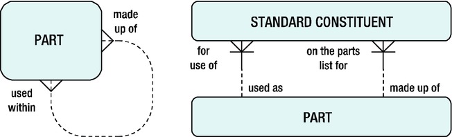
Figure 9-1. A solution for the “bill of materials” problem
Notice that for the solution on the left-hand side, if you replaced the entity name PART with THING, and you replaced the two relationship descriptions with “related to,” then you would have the ultimate in generic data models! Although this book is not about database design, consider this joke as a serious warning: don’t make your data models overly generic.
Even if hierarchical data structures are correctly translated into relational tables, the retrieval of such structures can still be quite challenging. We have an example of a simple hierarchical relationship in our sample tables: the management structure in the EMPLOYEES table is implemented with the MGR column and its foreign key constraint to the EMPNO column of the same table.
![]() Note In hierarchical structures, it is common practice to refer to parent rows and children rows. Another common (and self-explanatory) terminology is using a tree metaphor by referring to root, branch, and leaf rows.
Note In hierarchical structures, it is common practice to refer to parent rows and children rows. Another common (and self-explanatory) terminology is using a tree metaphor by referring to root, branch, and leaf rows.
START WITH and CONNECT BY
Oracle SQL supports a number of operators—and pseudo columns populated by those operators—to facilitate queries against hierarchical data. Let’s look at a simple example first, shown in Listing 9-19.
Listing 9-19. Hierarchical Query Example
select  ename, LEVEL
from    employees
START   WITH mgr is null
CONNECT BY NOCYCLE PRIOR empno = mgr;

ENAME       LEVEL
-------- --------
KING            1
JONES           2
SCOTT           3
ADAMS           4
FORD            3
SMITH           4
BLAKE           2
ALLEN           3
WARD            3
MARTIN          3
TURNER          3
JONES           3
CLARK           2
MILLER          3
The START WITH and CONNECT BY clauses allow you to do the following:
- Identify a starting point (root) for the tree structure.
- Specify how you can walk up or down the tree structure from any row.
The START WITH and CONNECT BY clauses must be specified after the WHERE clause (if any) and before the GROUP BY clause (if any).
![]() Note It is your own responsibility to indicate the correct starting point (or root) for the hierarchy. Listing 9-19 uses the predicate, MGR is null, as a condition, because we know that the null value in the MGR column has a special meaning. The Oracle DBMS treats each row for which the START WITH condition evaluates to TRUE as root for a separate tree structure; that is, you can define multiple tree structures within the context of a single query.
Note It is your own responsibility to indicate the correct starting point (or root) for the hierarchy. Listing 9-19 uses the predicate, MGR is null, as a condition, because we know that the null value in the MGR column has a special meaning. The Oracle DBMS treats each row for which the START WITH condition evaluates to TRUE as root for a separate tree structure; that is, you can define multiple tree structures within the context of a single query.
The NOCYCLE keyword in the CONNECT BY clause is optional; however, if you omit NOCYCLE, you risk ending up in a loop. If that happens, the Oracle DBMS returns the following error message:
ORA-01436: CONNECT BY loop in user data
Conversely, one example of a looping condition that could take place is the scenario where the employee with an EMPNO value of 1 has a MGR value of 2. And the employee with an EMPNO value of 2 has a MGR value of 1. This could very well represent a logical data error. However, using the NOCYCLE keyword in such a situation would mask the error. You would not receive the Oracle DBMS error ORA-01436, but you could receive unexpected results in your query output.
Our EMPLOYEES table doesn’t contain any cyclic references, but specifying NOCYCLE never hurts.
Pay special attention to the placement of the PRIOR operator. The PRIOR operator always points to the parent row. In Listing 9-19, PRIOR is placed before EMPNO, so we are able to find parent rows by starting from the MGR column value of the current row and then searching the EMPNO column values in all other rows for a match. If you put PRIOR in the wrong place, you define hierarchical relationships in the opposite direction. Just see what happens in Listing 9-19 if you change the fourth line to CONNECT BY PRIOR MGR = EMPNO or to CONNECT BY EMPNO = PRIOR MGR.
At first sight, the result in Listing 9-19 is not very impressive, since you just get a list of employee names, followed by a number. And if we had omitted LEVEL from the SELECT clause, the result would have been completely trivial. However, many things happened behind the scenes. We just have not exploited the full benefits yet.
LEVEL, CONNECT_BY_ISCYCLE, and CONNECT_BY_ISLEAF
As a consequence of using START WITH and CONNECT BY, the Oracle DBMS assigns several pseudo column values to every row. Listing 9-19 showed a first example of such a pseudo column: LEVEL. You can use these pseudo column values for many purposes, for example, to filter specific rows in the WHERE clause or to enhance the readability of your results in the SELECT clause.
The following are the hierarchical pseudo columns:
- LEVEL: The level of the row in the tree structure.
- CONNECT_BY_ISCYCLE: The value is 1 for each row with achild that is also a parent of the same row (that is, you have a cyclic reference); otherwise, the value is 0.
- CONNECT_BY_ISLEAF: The value is 1 if the row is aleaf; otherwise, the value is 0. Since a leaf is the last or lowest member of the hierarchy it does not have any children.
Listing 9-20 illustrates an example using the LEVEL pseudo column combined with the LPAD function, adding indentation to highlight the hierarchical query results.
Listing 9-20. Enhancing Readability with the LPAD Function
select  lpad(' ',2*level-1)||ename as ename
from    employees
start   with mgr is null
connect by nocycle prior empno = mgr;

ENAME
-----------------
 KING
   JONES
     SCOTT
       ADAMS
     FORD
       SMITH
   BLAKE
     ALLEN
     WARD
     MARTIN
     TURNER
     JONES
   CLARK
     MILLER
CONNECT_BY_ROOT and SYS_CONNECT_BY_PATH
If you use START WITH and CONNECT BY to define a hierarchical query, you can use two interesting hierarchical operators in the SELECT clause:
- CONNECT_BY_ROOT: Thisperator allows you to connect each row (regardless of its level in the tree structure) with its own root.
- SYS_CONNECT_BY_PATH: This function allows you to display the full path from the current row to its root.
See Listing 9-21 for an example of using both operators. Note that the START WITH clause in Listing 9-21 creates three separate tree structures: one for each manager.
Listing 9-21. Using CONNECT_BY_ROOT and SYS_CONNECT_BY_PATH
select  ename
,       connect_by_root ename            as manager
,       sys_connect_by_path(ename,' > ') as full_path
from    employees
start   with job = 'MANAGER'
connect by prior empno = mgr;

ENAME    MANAGER  FULL_PATH
-------- -------- -------------------------
JONES    JONES     > JONES
SCOTT    JONES     > JONES > SCOTT
ADAMS    JONES     > JONES > SCOTT > ADAMS
FORD     JONES     > JONES > FORD
SMITH    JONES     > JONES > FORD > SMITH
BLAKE    BLAKE     > BLAKE
ALLEN    BLAKE     > BLAKE > ALLEN
WARD     BLAKE     > BLAKE > WARD
MARTIN   BLAKE     > BLAKE > MARTIN
TURNER   BLAKE     > BLAKE > TURNER
JONES    BLAKE     > BLAKE > JONES
CLARK    CLARK     > CLARK
MILLER   CLARK     > CLARK > MILLER
You can specify additional conditions in the CONNECT BY clause, thus eliminating entire subtree structures. Note the important difference with conditions in the WHERE clause: those conditions filter only individual rows. See the Oracle SQL Language Reference (http://docs.oracle.com/cd/E16655_01/server.121/e17209/toc.htm) for more details and examples.
Hierarchical Query Result Sorting
If you want to sort the results of hierarchical queries, and you use a regular ORDER BY clause, the carefully constructed hierarchical tree gets disturbed in most cases. In such cases, you can use the SIBLINGS option of the ORDER BY clause. This option doesn’t destroy the hierarchy of the rows in the result. See Listings 9-22 and 9-23 for an example, and watch what happens with the query result if we remove the SIBLINGS option. Listing 9-22 displays the use of siblings. Listing 9-23 shows the results without that keyword.
Listing 9-22. Results When Ordering By Siblings
select  ename
,       sys_connect_by_path(ename,'|') as path
from    employees
start   with mgr is null
connect by prior empno = mgr
order   SIBLINGS by ename;

ENAME    PATH
-------- -----------------------------
KING     |KING
BLAKE    |KING|BLAKE
ALLEN    |KING|BLAKE|ALLEN
JONES    |KING|BLAKE|JONES
MARTIN   |KING|BLAKE|MARTIN
TURNER   |KING|BLAKE|TURNER
WARD     |KING|BLAKE|WARD
CLARK    |KING|CLARK
MILLER   |KING|CLARK|MILLER
JONES    |KING|JONES
FORD     |KING|JONES|FORD
SMITH    |KING|JONES|FORD|SMITH
SCOTT    |KING|JONES|SCOTT
ADAMS    |KING|JONES|SCOTT|ADAMS
Listing 9-23. Results from a Standard ORDER BY Clause
select  ename
,       sys_connect_by_path(ename,'|') as path
from    employees
start   with mgr is null
connect by prior empno = mgr
order   by ename;

ENAME    PATH
-------- ------------------------------
ADAMS    |KING|JONES|SCOTT|ADAMS
ALLEN    |KING|BLAKE|ALLEN
BLAKE    |KING|BLAKE
CLARK    |KING|CLARK
FORD     |KING|JONES|FORD
JONES    |KING|JONES
JONES    |KING|BLAKE|JONES
KING     |KING
MARTIN   |KING|BLAKE|MARTIN
MILLER   |KING|CLARK|MILLER
SCOTT    |KING|JONES|SCOTT
SMITH    |KING|JONES|FORD|SMITH
TURNER   |KING|BLAKE|TURNER
WARD     |KING|BLAKE|WARD
9.6 Analytic Functions
This section introduces the concept of analytic functions, which are a very powerful part of the ANSI/ISO SQL standard syntax. Analytic functions enable you to produce derived attributes that would otherwise be very complicated to achieve in SQL. Rankings, Top N reports, and running totals are all possible using analytical SQL. In fact they are not just possible, but the resulting statement is clearer and performance is usually better than with multiple-pass statements.
Earlier in this chapter, in Section 9.2, you saw how subqueries in the SELECT clause allow you to add derived attributes to the SELECT clause of your queries. Analytic functions provide similar functionality, though with enhanced statement clarity and improved performance.
![]() Note You should always test the performance of any analytic functions on production-like data sets. These functions are designed for use with large data sets and are optimized accordingly. When these functions are used with small data sets, as you might find in development, they may not perform as well as other statements. Do not conclude that the performance is unacceptable until you test with appropriately sized data sets.
Note You should always test the performance of any analytic functions on production-like data sets. These functions are designed for use with large data sets and are optimized accordingly. When these functions are used with small data sets, as you might find in development, they may not perform as well as other statements. Do not conclude that the performance is unacceptable until you test with appropriately sized data sets.
Let’s take a look at a simple query, reporting the salary ranking by department for all employees. Listing 9-24 displays the query and the results.
Listing 9-24. Ranking Employee Salary Using Multiple Table Access
SELECT e1.deptno, e1.ename, e1.msal,
       (SELECT COUNT(1)
        FROM employees e2
        WHERE  e2.msal > e1.msal)+1 sal_rank
FROM employees e1
ORDER BY e1.msal DESC;

DEPTNO ENAME      MSAL SAL_RANK
------ -------- ------ --------
    10 KING       5000        1
    20 FORD       3000        2
    20 SCOTT      3000        2
    20 JONES      2975        4
    30 BLAKE      2850        5
    10 CLARK      2450        6
    30 ALLEN      1600        7
    30 TURNER     1500        8
    10 MILLER     1300        9
    30 WARD       1250       10
    30 MARTIN     1250       10
    20 ADAMS      1100       12
    30 JONES       800       13
    20 SMITH       800       13
This version of the query doesn’t use an analytic function. It uses a more traditional, subquery-based approach to the problem of ranking. The problem is that the subquery essentially represents an additional query to the employees table for each row that is being ranked. If the employees table is large, this can result in a large number of data reads and consume minutes, perhaps hours, of response time. Listing 9-25 generates the same report using the analytic function RANK.
Listing 9-25. Ranking Employee Salary Using Analytic Funcions
SELECT e1.deptno, e1.ename, e1.msal,
       RANK() OVER (ORDER BY e1.msal DESC) sal_rank
FROM employees e1
ORDER BY e1.msal DESC;

DEPTNO ENAME      MSAL SAL_RANK
------ -------- ------ --------
    10 KING       5000        1
    20 FORD       3000        2
    20 SCOTT      3000        2
    20 JONES      2975        4
    30 BLAKE      2850        5
    10 CLARK      2450        6
    30 ALLEN      1600        7
    30 TURNER     1500        8
    10 MILLER     1300        9
    30 WARD       1250       10
    30 MARTIN     1250       10
    20 ADAMS      1100       12
    30 JONES       800       13
    20 SMITH       800       13
Using the analytic function creates a statement that is simpler and self documenting. Figure 9-2 illustrates the basic format of the analytic function.
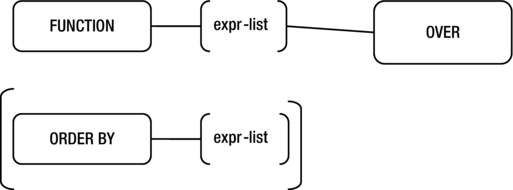
Figure 9-2. Basic syntax for analytic functions
The use of the term OVER indicates an analytic function, something you need to keep in mind as there are analytic functions with the same names as regular functions. For example, the analytic functions SUM and AVG have the same names as their non-analytic counterparts.
A key clause is ORDER BY. This indicates the order in which the functions are applied. In the preceding example, RANK is applied according to the employee salary. Remember that the default for ORDER BY is ascending, smallest to largest, so you have to specify the keyword DESC, for descending, to sort from largest to smallest. The ORDER BY clause must come last in the analytic function.
ORDER BY VERSUS ORDER BY
Do take care to remember that the statement ORDER BY and the function ORDER BY are independent of each other. If you place another clause after the ORDER BY in a function call, you receive the following rather cryptic error message:
PARTITION BY empno) prev_sal
*
ERROR at line 6:
ORA-00907: missing right parenthesis
The ORDER BY in a function call applies only to the evaluation of that function and has nothing to do with sorting the rows to be returned by the statement.
Partitions
A partition is a set of rows defined by data values in the result set. The default partition for any function is the entire result set. You can have one partition clause per function, though it may be a composite partition, including more than one data value. The PARTITION BY clause must come before the ORDER BY clause. Figure 9-3 illustrates the basic format of the analytic function using a PARTITION.
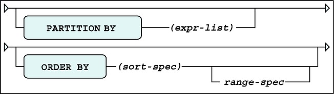
Figure 9-3. Analytic function partitioning syntax
When a partition is defined, the rows belonging to each partition are grouped together and the function is applied within each group. In Listing 9-26, one RANK is for the entire company and the second RANK is within each department.
Listing 9-26. Ranking Employee Salary Within the Company and Department
SELECT e1.deptno, e1.ename, e1.msal,
       RANK() OVER (ORDER BY e1.msal DESC) sal_rank,
       RANK() OVER (PARTITION BY e1.deptno
                    ORDER BY e1.msal DESC) dept_sal_rank
FROM employees e1
ORDER BY e1.deptno ASC, e1.msal DESC;

DEPTNO ENAME      MSAL SAL_RANK DEPT_SAL_RANK
------ -------- ------ -------- -------------
    10 KING       5000        1             1
    10 CLARK      2450        6             2
    10 MILLER     1300        9             3
    20 FORD       3000        2             1
    20 SCOTT      3000        2             1
    20 JONES      2975        4             3
    20 ADAMS      1100       12             4
    20 SMITH       800       13             5
    30 BLAKE      2850        5             1
    30 ALLEN      1600        7             2
    30 TURNER     1500        8             3
    30 MARTIN     1250       10             4
    30 WARD       1250       10             4
    30 JONES       800       13             6
Functions cannot span a partition boundary, which is the condition where the partition value changes. When the DEPTNO changes value, the RANK() with the PARTITION BY E1.DEPTNO resets to 1. Other functions, such as LAG or LEAD, cannot reference rows outside the current row’s partition. Listing 9-27 shows how to reference data in rows other than the current row.
Listing 9-27. Listing Employee Current and Previous Salaries
SELECT     empno
      ,    begindate
      ,    enddate
      ,    msal
      ,    LAG(msal) OVER (PARTITION BY empno
                           ORDER BY begindate) prev_sal
FROM       history
ORDER BY   empno, begindate;

EMPNO BEGINDATE ENDDATE     MSAL PREV_SAL
----- --------- --------- ------ --------
 7369 01-JAN-00 01-FEB-00    950
 7369 01-FEB-00              800      950
 7499 01-JUN-88 01-JUL-89   1000
 7499 01-JUL-89 01-DEC-93   1300     1000
 7499 01-DEC-93 01-OCT-95   1500     1300
 7499 01-OCT-95 01-NOV-99   1700     1500
 7499 01-NOV-99             1600     1700
Here is an example of using the LAG function to calculate the raise someone received. The LAG function returns the same datatype as the expression, in this case a number, so it can be used in an expression itself. Listing 9-28 illustrates how to use the current and previous salaries to calculate the raise in pay.
Listing 9-28. Using LAG to Calculate a Raise
SELECT     empno
      ,    begindate
      ,    enddate
      ,    msal
      ,    LAG(msal) OVER (PARTITION BY empno
                           ORDER BY begindate) prev_sal
      ,    msal - LAG(msal) OVER (PARTITION BY empno
                                  ORDER BY begindate) raise
FROM       history
ORDER BY   empno, begindate;

EMPNO BEGINDATE ENDDATE     MSAL PREV_SAL  RAISE
----- --------- --------- ------ -------- ------
 7369 01-JAN-00 01-FEB-00    950
 7369 01-FEB-00              800      950   -150
 7499 01-JUN-88 01-JUL-89   1000
 7499 01-JUL-89 01-DEC-93   1300     1000    300
 7499 01-DEC-93 01-OCT-95   1500     1300    200
 7499 01-OCT-95 01-NOV-99   1700     1500    200
 7499 01-NOV-99             1600     1700   -100
Notice that the LAG(msal) does not look backward when the EMPNO changes from 7369 to 7499. A common mistake is to not specify the correct PARTITION BY and the function returns data that you did not intend. It is always a good practice to manually and visually validate the data as you are writing the query.
Function Processing
There are three distinct phases in which statements containing analytic functions are processed. They are shown in the following list. The list also shows the steps within each phase.
It is very important to keep in mind that all of the data retrieval for the query occurs before the analytic functions are executed. It is important to keep this in mind as it restricts what you can do with analytic functions in a single query.
- Execute the query clauses, except
ORDER BY
   SELECT
   WHERE/joins
GROUP BY/HAVING - Execute the analytic function. This phase occurs once for every function in the statement.
     Define the partition(s)
Order the data within each partition
Define the window
Apply function - Sort query results per the statement’s ORDER BY clause.
Since analytic functions are not processed until after the WHERE clause has been evaluated, the use of analytic functions in the WHERE clause is not supported. (Similarly, you cannot apply analytic functions in a HAVING clause). If you try to use one in the WHERE clause, you receive a somewhat cryptic error, as shown in Listing 9-29.
Listing 9-29. Error Resulting from Analytic Function Placed in a WHERE Clause
SELECT     ename
      ,    job
      ,    mgr
      ,    msal
      ,    DENSE_RANK() OVER (ORDER BY msal DESC) sal_rank
FROM       employees
WHERE      (DENSE_RANK() OVER (ORDER BY msal DESC)) <= 3
ORDER BY   msal DESC;

WHERE      (DENSE_RANK() OVER (ORDER BY msal DESC)) <= 3
            *
ERROR at line 7:
ORA-30483: window  functions are not allowed here
If you want to filter records based on an analytic function, you will need to create a subquery that uses the function and then use the resulting value to filter on as shown in Listing 9-30.
Listing 9-30. Using a Factored Subquery to Filter on an Analytic Function
WITH ranked_salaries AS
( SELECT     ename
        ,    job
        ,    mgr
        ,    msal
        ,    DENSE_RANK() OVER (ORDER BY msal DESC) sal_rank
  FROM       employees
 )
SELECT     ename
      ,    job
      ,    mgr
      ,    msal
      ,    sal_rank
FROM       ranked_salaries
WHERE      sal_rank <= 3
ORDER BY   msal DESC;

ENAME    JOB        MGR   MSAL SAL_RANK
-------- -------- ----- ------ --------
KING     DIRECTOR         5000        1
SCOTT    TRAINER   7566   3000        2
FORD     TRAINER   7566   3000        2
JONES    MANAGER   7839   2975        3
Analytic functions enable you to reference other rows and group data in different ways. This will require that you begin to look at your data and query requirements in a more complex way, which will be your biggest challenge in leveraging analytic functions. Begin to look for opportunities to use these functions as you get more familiar with them. When you find yourself accessing the same table several times in a query, this might indicate that the information you desire can be derived using analytic functions.
While the specific functions are documented in the Oracle SQL Language Reference (http://docs.oracle.com/cd/E16655_01/server.121/e17209/toc.htm), a more thorough treatment of the functions, partitions, and windows is given in the Oracle Data Warehousing and Business Intelligence Reference (http://docs.oracle.com/cd/E16655_01/nav/portal_6.htm).
9.7 Row Limiting
Oracle Database version 12c allows Top-N queries to employ simpler syntax with the use of the row limiting clause, which allows you to limit the rows returned by a query. This can greatly simplify the syntax required for providing you with the ability to page through an ordered set. Listing 9-31 displays two queries for comparison purposes: one that queries from the EMPLOYEES table with no row limiting applied, and one that queries the EMPLOYEES table with the row limiting FETCH FIRST and ROWS ONLY clauses employed.
Listing 9-31. A Comparison of Two Queries: One Without Row Limiting Applied and One with Row Limiting Applied
SQL> select empno, ename||','||init name, job, msal
  2    from employees
  3  order by msal desc, name;

EMPNO NAME           JOB      MSAL
----- -------------- -------- ------
 7839 KING,CC        DIRECTOR   5000
 7902 FORD,MG        TRAINER    3000
 7788 SCOTT,SCJ      TRAINER    3000
 7566 JONES,JM       MANAGER    2975
 7698 BLAKE,R        MANAGER    2850
 7782 CLARK,AB       MANAGER    2450
 7499 ALLEN,JAM      SALESREP   1600
 7844 TURNER,JJ      SALESREP   1500
 7934 MILLER,TJA     ADMIN      1300
 7654 MARTIN,P       SALESREP   1250
 7521 WARD,TF        SALESREP   1250
 7876 ADAMS,AA       TRAINER    1100
 7900 JONES,R        ADMIN       800
 7369 SMITH,N        TRAINER     800

14 rows selected.

SQL> select empno, ename||','||init name, job, msal
  2    from employees
  3  order by msal desc, name
  4  FETCH FIRST 5 ROWS ONLY;

EMPNO NAME           JOB      MSAL
----- -------------- -------- ------
 7839 KING,CC        DIRECTOR   5000
 7902 FORD,MG        TRAINER    3000
 7788 SCOTT,SCJ      TRAINER    3000
 7566 JONES,JM       MANAGER    2975
 7698 BLAKE,R        MANAGER    2850

5 rows selected.
Notice how with just a few extra keywords, FETCH FIRST 5 ROWS ONLY, the query is limited to the Top-N records we are interested in. This is a syntactical simplification over, for example, the RANK and DENSE_RANK analytic functions illustrated in Section 9.6. This is not to say that RANK and DENSE_RANK should not be used. (I am a huge fan of analytic functions.) This is simply a statement that many Top-N queries that are interested in, say, fetching the first five rows, and maybe the next five rows, for example, could make good use of the row limiting clause syntax available in Oracle Database version 12c.
The FETCH clause specifies the number of rows or percentage of rows to return. Comparing the second query with the first query, you can see that the omission of this clause results in all rows being returned. The second query fetches only the top five salary earners from the EMPLOYEES table. To then fetch the next top five salary earners, consider the query in Listing 9-32.
Listing 9-32. A Query That Uses the OFFSET and FETCH NEXT Options of the Row Limiting Clause
SQL> select empno, ename||','||init name, job, msal
  2    from employees
  3  order by msal desc, name
  4  OFFSET 5 ROWS FETCH NEXT 5 ROWS ONLY;

EMPNO NAME           JOB      MSAL
----- -------------- -------- ------
 7782 CLARK,AB       MANAGER    2450
 7499 ALLEN,JAM      SALESREP   1600
 7844 TURNER,JJ      SALESREP   1500
 7934 MILLER,TJA     ADMIN      1300
 7654 MARTIN,P       SALESREP   1250

5 rows selected.
The differences between the query in Listing 9-32 and the second query in Listing 9-31 are the OFFSET and FETCH NEXT clauses. The OFFSET clause specifies the number of rows to skip before the row limiting begins. The way to look at this is to read it as “skip the first five salary earners, and return the next five salary earners only.” Notice how there are actually two employees who earn a salary value of 1250 (first query in Listing 9-31). What if it were important to you to keep such records for employees with the same salary value together (similar to the concept of widows and orphans control in typesetting)? Listing 9-33 provides an example of the type of query you could write to keep similar values together while employing row limiting syntax.
Listing 9-33. A Query That Uses the WITH TIES Option of the Row Limiting Clause
SQL> select empno, ename||','||init name, job, msal
  2    from employees
  3  order by msal desc
  4  OFFSET 5 ROWS FETCH NEXT 5 ROWS WITH TIES;

EMPNO NAME           JOB      MSAL
----- -------------- -------- ------
 7782 CLARK,AB       MANAGER    2450
 7499 ALLEN,JAM      SALESREP   1600
 7844 TURNER,JJ      SALESREP   1500
 7934 MILLER,TJA     ADMIN      1300
 7521 WARD,TF        SALESREP   1250
 7654 MARTIN,P    SALESREP   1250

6 rows selected.
Note that even though the query in Listing 9-33 requested five rows, because it employed the WITH TIES option (NEXT 5 ROWS WITH TIES), instead of the ONLY option (NEXT 5 ROWS ONLY), six rows are actually returned. This is because the row limiting clause sorts the data according to the ORDER BY clause, and then sifts through the records to return only those records you’ve requested. Now we requested that the sort criteria be the MSAL value in descending order. We also requested that the first five records be skipped and not be returned as part of our data set. Then we stated that if five records are included in our result set but the last record actually has the same value for MSAL as another record(s) that is not currently part of our result set, then that record(s) should be included as well.
Note that if this query had used the same ORDER BY clause as that which we used in Listing 9-32, then only five records would have been returned as the entirety of the ORDER BY clause, both the MSAL and NAME values, would be evaluated. Only if the Oracle DBMS found other records with the same combination of MSAL and NAME values would it return extra records (beyond the specified limit of five).
This section covers some Oracle-specific extensions to the SQL language. Although they might appear slightly off topic, the flashback features are simply too valuable to remain uncovered in this book.
In Chapter 6, we talked about the concept of read consistency. Read consistency means that your SQL statements always get a consistent view of the data, regardless of what other database users or applications do with the same data at the same time. The Oracle DBMS provides a snapshot of the data at the point in time when the statement execution began. In the same chapter, you also saw that you can change your session to be READ ONLY so that your query results depend on the data as it was at the beginning of your session.
The Oracle DBMS has its methods to achieve this, without using any locking techniques affecting other database users or applications. How this is done is irrelevant for this book. This section shows some interesting ways to use the same technique, by stating explicitly in your queries that you want to go back in time.
![]() Note The flashback query feature may need some configuration efforts before you can use it. This is the task of a database administrator. Therefore, it is not covered in this book. See the Oracle documentation for more details.
Note The flashback query feature may need some configuration efforts before you can use it. This is the task of a database administrator. Therefore, it is not covered in this book. See the Oracle documentation for more details.
Before we begin our flashback query experiments, we first create a temporary copy of the EMPLOYEES table, as shown in Listing 9-34. (The listing is generated using SQL*Plus). This allows us to perform various experiments without destroying the contents of the real EMPLOYEES table. We also change the NLS_TIMESTAMP_FORMAT parameter with the ALTER SESSION command to influence how timestamp values are displayed on the screen.
Listing 9-34. Preparing for the Flashback Examples
SQL> create table e as select * from employees;
Table created.

SQL> alter session set nls_timestamp_format='DD-MON-YYYY HH24:MI:SS.FF3';
Session altered.

SQL> select localtimestamp as table_created from dual;
TABLE_CREATED
------------------------------------------------------
01-OCT-2004 10:53:42.746

SQL> update e set msal = msal + 10;
14 rows updated.
SQL> commit;
Commit complete.

SQL> select localtimestamp as after_update_1 from dual;
AFTER_UPDATE_1
-------------------------------------------------------
01-OCT-2004 10:54:26.138

SQL> update e set msal = msal - 20 where  deptno = 10;
3 rows updated.
SQL> commit;
Commit complete.

SQL> select localtimestamp as after_update_2 from dual;
AFTER_UPDATE_2
-------------------------------------------------------
01-OCT-2004 10:54:42.602

SQL> delete from e where  deptno <= 20;
8 rows deleted.
SQL> commit;
Commit complete.

SQL> select localtimestamp as now            from dual;
NOW
-------------------------------------------------------
01-OCT-2004 10:55:25.623

SQL>
![]() Tip Don’t execute these four steps too quickly in a row. You should take some time in between the steps. This makes it much easier during your experiments to go back to a specific point in time.
Tip Don’t execute these four steps too quickly in a row. You should take some time in between the steps. This makes it much easier during your experiments to go back to a specific point in time.
AS OF
Listings 9-35 to 9-37 show a first example of a flashback query. First, we select the current situation with a regular query (Listing 9-35). Then we use the AS OF TIMESTAMP option in the FROM clause to go back in time (Listing 9-36). Finally, we look at what happens when you try to go back in time beyond the amount of historical data that Oracle maintains (Listing 9-37). As illustrated in examples in earlier chapters, we use the SQL*Plus ampersand (&) substitution trick, which allows us to repeat the query conveniently with different timestamp values.
Listing 9-35. Evaluating the Current Situation
select empno, ename, deptno, msal
from   e;

   EMPNO ENAME      DEPTNO     MSAL
-------- -------- -------- --------
    7499 ALLEN          30     1610
    7521 WARD           30     1260
    7654 MARTIN         30     1260
    7698 BLAKE          30     2860
    7844 TURNER         30     1510
    7900 JONES          30      810
Listing 9-36. Querying as of Some Point in the Past
select empno, ename, deptno, msal
from   e
       AS OF TIMESTAMP to_timestamp('01-OCT-2004 10:53:47.000'),

   EMPNO ENAME      DEPTNO     MSAL
-------- -------- -------- --------
    7369 SMITH          20      800
    7499 ALLEN          30     1600
    7521 WARD           30     1250
    7566 JONES          20     2975
    7654 MARTIN         30     1250
    7698 BLAKE          30     2850
    7782 CLARK          10     2450
    7788 SCOTT          20     3000
    7839 KING           10     5000
    7844 TURNER         30     1500
    7876 ADAMS          20     1100
    7900 JONES          30      800
    7902 FORD           20     3000
    7934 MILLER         10     1300
Listing 9-37. Querying for a Point Too Far Back in Time
select empno, ename, deptno, msal
from   e
       AS OF TIMESTAMP to_timestamp('01-OCT-2004 10:53:42.000'),
       *
ERROR at line 2:
ORA-01466: unable to read data - table definition has changed
Of course, the timestamps to be used in Listing 9-35 depend on the timing of your experiments. Choose appropriate timestamps if you want to test these statements yourself. If you executed the steps of Listing 9-34 with some decent time intervals (as suggested), you have enough appropriate candidate values to play with.
The Oracle error message at the bottom of Listing 9-37 indicates that this query is trying to go back too far in time. In this case, table E didn’t even exist. Data definition changes (ALTER TABLE E ...) may also prohibit flashback queries, as suggested by the error message text.
VERSIONS BETWEEN
In Listing 9-38, we go one step further, using the VERSIONS BETWEEN operator. Now we get the complete history of the rows—that is, as far as the Oracle DBMS is able to reconstruct them.
Listing 9-38. Flashback Example: VERSIONS BETWEEN Syntax
break on empno

select empno, msal
,      versions_starttime
,      versions_endtime
from   e
      versions between timestamp minvalue and maxvalue
where  deptno = 10
order  by empno, versions_starttime nulls first;

   EMPNO     MSAL VERSIONS_STARTTIME        VERSIONS_ENDTIME
-------- -------- ------------------------- -------------------------
    7782     2450                           01-OCT-2004 10:54:23.000
             2460 01-OCT-2004 10:54:23.000  01-OCT-2004 10:54:41.000
             2440 01-OCT-2004 10:54:41.000  01-OCT-2004 10:55:24.000
             2440 01-OCT-2004 10:55:24.000
    7839     5000                           01-OCT-2004 10:54:23.000
             5010 01-OCT-2004 10:54:23.000  01-OCT-2004 10:54:41.000
             4990 01-OCT-2004 10:54:41.000  01-OCT-2004 10:55:24.000
             4990 01-OCT-2004 10:55:24.000
    7934     1300                           01-OCT-2004 10:54:23.000
             1310 01-OCT-2004 10:54:23.000  01-OCT-2004 10:54:41.000
             1290 01-OCT-2004 10:54:41.000  01-OCT-2004 10:55:24.000
             1290 01-OCT-2004 10:55:24.000
By using the VERSIONS BETWEEN operator in the FROM clause, you introduce several additional pseudo columns, such as VERSIONS_STARTTIME and VERSIONS_ENDTIME. You can use these pseudo columns in your queries.
By using the correct ORDER BY clause (watch the NULLS FIRST clause in Listing 9-38), you get a complete historical overview. You don’t see a start time for the three oldest salary values because you created the rows too long ago, and you don’t see an end time for the last value because it is the current salary value.
FLASHBACK TABLE
In Chapter 7, you learned that you can rescue an inadvertently dropped table from the recycle bin with the FLASHBACK TABLE command. Listing 9-39 shows another example of this usage.
Listing 9-39. Using FLASHBACK TABLE . . . TO BEFORE DROP
drop table e;
Table dropped.

SQL> show recyclebin;
ORIGINAL NAME RECYCLEBIN NAME                OBJECT TYPE  DROP TIME
------------- ------------------------------ ------------ -------------------
E             BIN$8lO2OsyQe0ngRQAAAAAAAQ==$0 TABLE        2014-02-13:19:16:05

flashback table e to before drop;
Flashback complete.

select * from e;

 EMPNO ENAME    INIT  JOB         MGR BDATE         MSAL   COMM DEPTNO
------ -------- ----- -------- ------ ----------- ------ ------ ------
  7499 ALLEN    JAM   SALESREP   7698 20-FEB-1961   1610    300     30
  7521 WARD     TF    SALESREP   7698 22-FEB-1962   1260    500     30
  7654 MARTIN   P     SALESREP   7698 28-SEP-1956   1260   1400     30
  7698 BLAKE    R     MANAGER    7839 01-NOV-1963   2860            30
  7844 TURNER   JJ    SALESREP   7698 28-SEP-1968   1510      0     30
  7900 JONES    R     ADMIN      7698 03-DEC-1969    810            30
You can go back to any point in time with the FLASHBACK TABLE command, as you can see in Listing 9-40. Note the following important difference: Listings 9-36 and 9-38 show queries against table E where you go back in time, but the FLASHBACK TABLE example in Listing 9-40 changes the database and restores table E to a given point in time.
Listing 9-40. Another FLASHBACK TABLE Example
select count(*) from e;
COUNT(*)
--------
6
flashback table e to timestamp to_timestamp('×tamp'),
Enter value for timestamp: 01-OCT-2004 10:54:00.000
Flashback complete.
select count(*) from e;
COUNT(*)
--------
14
It is not always possible to go back in time with one table using the FLASHBACK TABLE command. For example, you could have constraints referring to other tables prohibiting such a change. See the Oracle SQL Language Reference (http://docs.oracle.com/cd/E16655_01/server.121/e17209/toc.htm) for more details about the FLASHBACKTABLE command.
9.9 Exercises
You can practice applying the advanced retrieval functions covered in this chapter in the following exercises. The answers are presented in Appendix B.
- It is normal practice that (junior) trainers always attend a course taught by a senior colleague before teaching that course themselves. For which trainer/course combinations did this happen?
- Actually, if the junior trainer teaches a course for the first time, that senior colleague (see the previous exercise) sits in the back of the classroom in a supporting role. Try to find these course/junior/senior combinations.
- Which employees never taught a course?
- Which employees attended all build courses (category BLD)? They are entitled to get a discount on the next course they attend.
- Provide a list of all employees having the same monthly salary and commission as (at least) one employee of Department 30. You are interested in only employees from other departments.
- Look again at Listings 9-3 and 9-4. Are they really logically equivalent? Just for testing purposes, search on a nonexisting job and execute both queries again. Explain the results.
- You saw a series of examples in this chapter about all employees that ever taught an SQL course (in Listings 9-9 through 9-11). How can you adapt these queries in such a way that they answer the negation of the same question (... all employees that never . . .)?
- Check out your solution for Exercise 4 in Chapter 8: “For all course offerings, list the course code, begin date, and number of registrations. Sort your results on the number of registrations, from high to low.” Can you come up with a more elegant solution now, without using an outer join?
- Who attended (at least) the same courses as employee 7788?
- Give the name and initials of all employees at the bottom of the management hierarchy, with a third column showing the number of management levels above them.