
Much of the programming work in data analysis and modeling is spent on data preparation: loading, cleaning, transforming, and rearranging. Sometimes the way that data is stored in files or databases is not the way you need it for a data processing application. Many people choose to do ad hoc processing of data from one form to another using a general purpose programming, like Python, Perl, R, or Java, or UNIX text processing tools like sed or awk. Fortunately, pandas along with the Python standard library provide you with a high-level, flexible, and high-performance set of core manipulations and algorithms to enable you to wrangle data into the right form without much trouble.
If you identify a type of data manipulation that isn’t anywhere in this book or elsewhere in the pandas library, feel free to suggest it on the mailing list or GitHub site. Indeed, much of the design and implementation of pandas has been driven by the needs of real world applications.
Data contained in pandas objects can be combined together in a number of built-in ways:
pandas.mergeconnects rows in DataFrames based on one or more keys. This will be familiar to users of SQL or other relational databases, as it implements database join operations.pandas.concatglues or stacks together objects along an axis.combine_firstinstance method enables splicing together overlapping data to fill in missing values in one object with values from another.
I will address each of these and give a number of examples. They’ll be utilized in examples throughout the rest of the book.
Merge or join
operations combine data sets by linking rows using one or more
keys. These operations are central to relational
databases. The merge function in
pandas is the main entry point for using these algorithms on your
data.
Let’s start with a simple example:
In [15]: df1 = DataFrame({'key': ['b', 'b', 'a', 'c', 'a', 'a', 'b'],
   ....:                  'data1': range(7)})

In [16]: df2 = DataFrame({'key': ['a', 'b', 'd'],
   ....:                  'data2': range(3)})

In [17]: df1        In [18]: df2
Out[17]:            Out[18]:
   data1 key           data2 key
0      0   b        0      0   a
1      1   b        1      1   b
2      2   a        2      2   d
3      3   c
4      4   a
5      5   a
6      6   b
This is an example of a many-to-one merge situation; the data
in df1 has multiple rows labeled
a and b, whereas df2 has only one row for each value in the
key column. Calling merge with these objects we obtain:
In [19]: pd.merge(df1, df2)
Out[19]:
   data1 key  data2
0      0   b      1
1      1   b      1
2      6   b      1
3      2   a      0
4      4   a      0
5      5   a      0
Note that I didn’t specify which column to join on. If not
specified, merge uses the overlapping
column names as the keys. It’s a good practice to specify explicitly,
though:
In [20]: pd.merge(df1, df2, on='key')
Out[20]:
   data1 key  data2
0      0   b      1
1      1   b      1
2      6   b      1
3      2   a      0
4      4   a      0
5      5   a      0
If the column names are different in each object, you can specify them separately:
In [21]: df3 = DataFrame({'lkey': ['b', 'b', 'a', 'c', 'a', 'a', 'b'],
   ....:                  'data1': range(7)})

In [22]: df4 = DataFrame({'rkey': ['a', 'b', 'd'],
   ....:                  'data2': range(3)})

In [23]: pd.merge(df3, df4, left_on='lkey', right_on='rkey')
Out[23]:
   data1 lkey  data2 rkey
0      0    b      1    b
1      1    b      1    b
2      6    b      1    b
3      2    a      0    a
4      4    a      0    a
5      5    a      0    a
You probably noticed that the 'c' and 'd'
values and associated data are missing from the result. By default
merge does an
'inner' join; the keys in the result are the
intersection. Other possible options are 'left',
'right', and 'outer'. The outer join takes the union of the
keys, combining the effect of applying both left and right joins:
In [24]: pd.merge(df1, df2, how='outer')
Out[24]:
   data1 key  data2
0      0   b      1
1      1   b      1
2      6   b      1
3      2   a      0
4      4   a      0
5      5   a      0
6      3   c    NaN
7    NaN   d      2
Many-to-many merges have well-defined though not necessarily intuitive behavior. Here’s an example:
In [25]: df1 = DataFrame({'key': ['b', 'b', 'a', 'c', 'a', 'b'],
   ....:                  'data1': range(6)})

In [26]: df2 = DataFrame({'key': ['a', 'b', 'a', 'b', 'd'],
   ....:                  'data2': range(5)})

In [27]: df1        In [28]: df2
Out[27]:            Out[28]:
   data1 key           data2 key
0      0   b        0      0   a
1      1   b        1      1   b
2      2   a        2      2   a
3      3   c        3      3   b
4      4   a        4      4   d
5      5   b

In [29]: pd.merge(df1, df2, on='key', how='left')
Out[29]:
    data1 key  data2
0       0   b      1
1       0   b      3
2       1   b      1
3       1   b      3
4       5   b      1
..    ...  ..    ...
6       2   a      0
7       2   a      2
8       4   a      0
9       4   a      2
10      3   c    NaN
[11 rows x 3 columns]
Many-to-many joins form the Cartesian product of the rows. Since
there were 3 'b' rows in the left
DataFrame and 2 in the right one, there are 6 'b' rows in the result. The join method only
affects the distinct key values appearing in the result:
In [30]: pd.merge(df1, df2, how='inner')
Out[30]:
   data1 key  data2
0      0   b      1
1      0   b      3
2      1   b      1
3      1   b      3
4      5   b      1
5      5   b      3
6      2   a      0
7      2   a      2
8      4   a      0
9      4   a      2
To merge with multiple keys, pass a list of column names:
In [31]: left = DataFrame({'key1': ['foo', 'foo', 'bar'],
   ....:                   'key2': ['one', 'two', 'one'],
   ....:                   'lval': [1, 2, 3]})

In [32]: right = DataFrame({'key1': ['foo', 'foo', 'bar', 'bar'],
   ....:                    'key2': ['one', 'one', 'one', 'two'],
   ....:                    'rval': [4, 5, 6, 7]})

In [33]: pd.merge(left, right, on=['key1', 'key2'], how='outer')
Out[33]:
  key1 key2  lval  rval
0  foo  one     1     4
1  foo  one     1     5
2  foo  two     2   NaN
3  bar  one     3     6
4  bar  two   NaN     7
To determine which key combinations will appear in the result depending on the choice of merge method, think of the multiple keys as forming an array of tuples to be used as a single join key (even though it’s not actually implemented that way).
Caution
When joining columns-on-columns, the indexes on the passed DataFrame objects are discarded.
A last issue to consider in merge operations is the treatment of
overlapping column names. While you can address the overlap manually
(see the later section on renaming axis labels), merge has a suffixes option for specifying strings to
append to overlapping names in the left and right DataFrame
objects:
In [34]: pd.merge(left, right, on='key1')
Out[34]:
  key1 key2_x  lval key2_y  rval
0  foo    one     1    one     4
1  foo    one     1    one     5
2  foo    two     2    one     4
3  foo    two     2    one     5
4  bar    one     3    one     6
5  bar    one     3    two     7

In [35]: pd.merge(left, right, on='key1', suffixes=('_left', '_right'))
Out[35]:
  key1 key2_left  lval key2_right  rval
0  foo       one     1        one     4
1  foo       one     1        one     5
2  foo       two     2        one     4
3  foo       two     2        one     5
4  bar       one     3        one     6
5  bar       one     3        two     7
See Table 7-1 for an argument
reference on merge. Joining on index
is the subject of the next section.
Table 7-1. merge function arguments
In some cases, the merge key or keys in a DataFrame will
be found in its index. In this case, you can pass left_index=True or right_index=True (or both) to indicate that
the index should be used as the merge key:
In [36]: left1 = DataFrame({'key': ['a', 'b', 'a', 'a', 'b', 'c'],
   ....:                   'value': range(6)})

In [37]: right1 = DataFrame({'group_val': [3.5, 7]}, index=['a', 'b'])

In [38]: left1        In [39]: right1
Out[38]:              Out[39]:
  key  value             group_val
0   a      0          a        3.5
1   b      1          b        7.0
2   a      2
3   a      3
4   b      4
5   c      5

In [40]: pd.merge(left1, right1, left_on='key', right_index=True)
Out[40]:
  key  value  group_val
0   a      0        3.5
2   a      2        3.5
3   a      3        3.5
1   b      1        7.0
4   b      4        7.0
Since the default merge method is to intersect the join keys, you can instead form the union of them with an outer join:
In [41]: pd.merge(left1, right1, left_on='key', right_index=True, how='outer')
Out[41]:
  key  value  group_val
0   a      0        3.5
2   a      2        3.5
3   a      3        3.5
1   b      1        7.0
4   b      4        7.0
5   c      5        NaN
With hierarchically-indexed data, things are a bit more complicated:
In [42]: lefth = DataFrame({'key1': ['Ohio', 'Ohio', 'Ohio', 'Nevada', 'Nevada'],
   ....:                    'key2': [2000, 2001, 2002, 2001, 2002],
   ....:                    'data': np.arange(5.)})

In [43]: righth = DataFrame(np.arange(12).reshape((6, 2)),
   ....:                    index=[['Nevada', 'Nevada', 'Ohio', 'Ohio', 'Ohio', 'Ohio'],
   ....:                           [2001, 2000, 2000, 2000, 2001, 2002]],
   ....:                    columns=['event1', 'event2'])

In [44]: lefth               In [45]: righth
Out[44]:                     Out[45]:
   data    key1  key2                     event1  event2
0     0    Ohio  2000        Nevada 2001       0       1
1     1    Ohio  2001               2000       2       3
2     2    Ohio  2002        Ohio   2000       4       5
3     3  Nevada  2001               2000       6       7
4     4  Nevada  2002               2001       8       9
                                    2002      10      11
In this case, you have to indicate multiple columns to merge on as a list (pay attention to the handling of duplicate index values):
In [46]: pd.merge(lefth, righth, left_on=['key1', 'key2'], right_index=True)
Out[46]:
   data    key1  key2  event1  event2
0     0    Ohio  2000       4       5
0     0    Ohio  2000       6       7
1     1    Ohio  2001       8       9
2     2    Ohio  2002      10      11
3     3  Nevada  2001       0       1

In [47]: pd.merge(lefth, righth, left_on=['key1', 'key2'],
   ....:          right_index=True, how='outer')
Out[47]:
   data    key1  key2  event1  event2
0     0    Ohio  2000       4       5
0     0    Ohio  2000       6       7
1     1    Ohio  2001       8       9
2     2    Ohio  2002      10      11
3     3  Nevada  2001       0       1
4     4  Nevada  2002     NaN     NaN
4   NaN  Nevada  2000       2       3
Using the indexes of both sides of the merge is also not an issue:
In [48]: left2 = DataFrame([[1., 2.], [3., 4.], [5., 6.]], index=['a', 'c', 'e'],
   ....:                  columns=['Ohio', 'Nevada'])

In [49]: right2 = DataFrame([[7., 8.], [9., 10.], [11., 12.], [13, 14]],
   ....:                    index=['b', 'c', 'd', 'e'], columns=['Missouri', 'Alabama'])

In [50]: left2         In [51]: right2
Out[50]:               Out[51]:
   Ohio  Nevada           Missouri  Alabama
a     1       2        b         7        8
c     3       4        c         9       10
e     5       6        d        11       12
                       e        13       14

In [52]: pd.merge(left2, right2, how='outer', left_index=True, right_index=True)
Out[52]:
   Ohio  Nevada  Missouri  Alabama
a     1       2       NaN      NaN
b   NaN     NaN         7        8
c     3       4         9       10
d   NaN     NaN        11       12
e     5       6        13       14
DataFrame has a more convenient join instance for
merging by index. It can also be used to combine together many DataFrame
objects having the same or similar indexes but non-overlapping columns.
In the prior example, we could have written:
In [53]: left2.join(right2, how='outer')
Out[53]:
   Ohio  Nevada  Missouri  Alabama
a     1       2       NaN      NaN
b   NaN     NaN         7        8
c     3       4         9       10
d   NaN     NaN        11       12
e     5       6        13       14
In part for legacy reasons (much earlier versions of pandas),
DataFrame’s join method performs a
left join on the join keys. It also supports joining the index of the
passed DataFrame on one of the columns of the calling DataFrame:
In [54]: left1.join(right1, on='key')
Out[54]:
  key  value  group_val
0   a      0        3.5
1   b      1        7.0
2   a      2        3.5
3   a      3        3.5
4   b      4        7.0
5   c      5        NaN
Lastly, for simple index-on-index merges, you can pass a list of
DataFrames to join as an alternative
to using the more general concat function
described below:
In [55]: another = DataFrame([[7., 8.], [9., 10.], [11., 12.], [16., 17.]],
   ....:                     index=['a', 'c', 'e', 'f'], columns=['New York', 'Oregon'])

In [56]: left2.join([right2, another])
Out[56]:
   Ohio  Nevada  Missouri  Alabama  New York  Oregon
a     1       2       NaN      NaN         7       8
c     3       4         9       10         9      10
e     5       6        13       14        11      12

In [57]: left2.join([right2, another], how='outer')
Out[57]:
   Ohio  Nevada  Missouri  Alabama  New York  Oregon
a     1       2       NaN      NaN         7       8
b   NaN     NaN         7        8       NaN     NaN
c     3       4         9       10         9      10
d   NaN     NaN        11       12       NaN     NaN
e     5       6        13       14        11      12
f   NaN     NaN       NaN      NaN        16      17
Another kind of data combination operation is
alternatively referred to as concatenation, binding, or stacking. NumPy
has a concatenate function for doing
this with raw NumPy arrays:
In [58]: arr = np.arange(12).reshape((3, 4))

In [59]: arr
Out[59]:
array([[ 0,  1,  2,  3],
       [ 4,  5,  6,  7],
       [ 8,  9, 10, 11]])

In [60]: np.concatenate([arr, arr], axis=1)
Out[60]:
array([[ 0,  1,  2,  3,  0,  1,  2,  3],
       [ 4,  5,  6,  7,  4,  5,  6,  7],
       [ 8,  9, 10, 11,  8,  9, 10, 11]])
In the context of pandas objects such as Series and DataFrame, having labeled axes enable you to further generalize array concatenation. In particular, you have a number of additional things to think about:
If the objects are indexed differently on the other axes, should the collection of axes be unioned or intersected?
Do the groups need to be identifiable in the resulting object?
Does the concatenation axis matter at all?
The concat function in pandas provides a
consistent way to address each of these concerns. I’ll give a number of
examples to illustrate how it works. Suppose we have three Series with
no index overlap:
In [61]: s1 = Series([0, 1], index=['a', 'b'])

In [62]: s2 = Series([2, 3, 4], index=['c', 'd', 'e'])

In [63]: s3 = Series([5, 6], index=['f', 'g'])
Calling concat with these
object in a list glues together the values and indexes:
In [64]: pd.concat([s1, s2, s3])
Out[64]:
a    0
b    1
c    2
d    3
e    4
f    5
g    6
dtype: int64
By default concat works along
axis=0, producing another Series. If
you pass axis=1, the result will
instead be a DataFrame (axis=1 is the
columns):
In [65]: pd.concat([s1, s2, s3], axis=1)
Out[65]:
    0   1   2
a   0 NaN NaN
b   1 NaN NaN
c NaN   2 NaN
d NaN   3 NaN
e NaN   4 NaN
f NaN NaN   5
g NaN NaN   6
In this case there is no overlap on the other axis, which as you
can see is the sorted union (the 'outer' join) of the indexes. You can instead
intersect them by passing join='inner':
In [66]: s4 = pd.concat([s1 * 5, s3])

In [67]: pd.concat([s1, s4], axis=1)      In [68]: pd.concat([s1, s4], axis=1, join='inner')
Out[67]:                                  Out[68]:
    0  1                                     0  1
a   0  0                                  a  0  0
b   1  5                                  b  1  5
f NaN  5
g NaN  6
You can even specify the axes to be used on the other axes with
join_axes:
In [69]: pd.concat([s1, s4], axis=1, join_axes=[['a', 'c', 'b', 'e']])
Out[69]:
    0   1
a   0   0
c NaN NaN
b   1   5
e NaN NaN
One issue is that the concatenated pieces are not identifiable in
the result. Suppose instead you wanted to create a hierarchical index on
the concatenation axis. To do this, use the keys argument:
In [70]: result = pd.concat([s1, s1, s3], keys=['one', 'two', 'three'])

In [71]: result
Out[71]:
one    a    0
       b    1
two    a    0
       b    1
three  f    5
       g    6
dtype: int64

# Much more on the unstack function later
In [72]: result.unstack()
Out[72]:
        a   b   f   g
one     0   1 NaN NaN
two     0   1 NaN NaN
three NaN NaN   5   6
In the case of combining Series along axis=1, the keys become the DataFrame column
headers:
In [73]: pd.concat([s1, s2, s3], axis=1, keys=['one', 'two', 'three'])
Out[73]:
   one  two  three
a    0  NaN    NaN
b    1  NaN    NaN
c  NaN    2    NaN
d  NaN    3    NaN
e  NaN    4    NaN
f  NaN  NaN      5
g  NaN  NaN      6
The same logic extends to DataFrame objects:
In [74]: df1 = DataFrame(np.arange(6).reshape(3, 2), index=['a', 'b', 'c'],
   ....:                 columns=['one', 'two'])

In [75]: df2 = DataFrame(5 + np.arange(4).reshape(2, 2), index=['a', 'c'],
   ....:                 columns=['three', 'four'])

In [76]: pd.concat([df1, df2], axis=1, keys=['level1', 'level2'])
Out[76]:
   level1       level2
      one  two   three  four
a       0    1       5     6
b       2    3     NaN   NaN
c       4    5       7     8
If you pass a dict of objects instead of a list, the dict’s keys
will be used for the keys
option:
In [77]: pd.concat({'level1': df1, 'level2': df2}, axis=1)
Out[77]:
   level1       level2
      one  two   three  four
a       0    1       5     6
b       2    3     NaN   NaN
c       4    5       7     8
There are a couple of additional arguments governing how the hierarchical index is created (see Table 7-2):
In [78]: pd.concat([df1, df2], axis=1, keys=['level1', 'level2'],
   ....:           names=['upper', 'lower'])
Out[78]:
upper  level1       level2
lower     one  two   three  four
a           0    1       5     6
b           2    3     NaN   NaN
c           4    5       7     8
A last consideration concerns DataFrames in which the row index is not meaningful in the context of the analysis:
In [79]: df1 = DataFrame(np.random.randn(3, 4), columns=['a', 'b', 'c', 'd'])

In [80]: df2 = DataFrame(np.random.randn(2, 3), columns=['b', 'd', 'a'])

In [81]: df1                                     In [82]: df2
Out[81]:                                         Out[82]:
          a         b         c         d                  b         d         a
0 -0.204708  0.478943 -0.519439 -0.555730        0  0.274992  0.228913  1.352917
1  1.965781  1.393406  0.092908  0.281746        1  0.886429 -2.001637 -0.371843
2  0.769023  1.246435  1.007189 -1.296221
In this case, you can pass ignore_index=True:
In [83]: pd.concat([df1, df2], ignore_index=True)
Out[83]:
          a         b         c         d
0 -0.204708  0.478943 -0.519439 -0.555730
1  1.965781  1.393406  0.092908  0.281746
2  0.769023  1.246435  1.007189 -1.296221
3  1.352917  0.274992       NaN  0.228913
4 -0.371843  0.886429       NaN -2.001637
Table 7-2. concat function arguments
Another data combination situation can’t be expressed as
either a merge or concatenation operation. You may have two datasets
whose indexes overlap in full or part. As a motivating example, consider
NumPy’s where function, which
expressed a vectorized if-else:
In [84]: a = Series([np.nan, 2.5, np.nan, 3.5, 4.5, np.nan],
   ....:            index=['f', 'e', 'd', 'c', 'b', 'a'])

In [85]: b = Series(np.arange(len(a), dtype=np.float64),
   ....:            index=['f', 'e', 'd', 'c', 'b', 'a'])

In [86]: b[-1] = np.nan

In [87]: a            In [88]: b            In [89]: np.where(pd.isnull(a), b, a)
Out[87]:              Out[88]:              Out[89]: array([ 0. ,  2.5,  2. ,
                                                             3.5,  4.5,  nan])
f    NaN              f     0
e    2.5              e     1
d    NaN              d     2
c    3.5              c     3
b    4.5              b     4
a    NaN              a   NaN
dtype: float64        dtype: float64
Series has a combine_first method,
which performs the equivalent of this operation plus data
alignment:
In [90]: b[:-2].combine_first(a[2:])
Out[90]:
a    NaN
b    4.5
c    3.0
d    2.0
e    1.0
f    0.0
dtype: float64
With DataFrames, combine_first naturally
does the same thing column by column, so you can think of it as
“patching” missing data in the calling object with data from the object
you pass:
In [91]: df1 = DataFrame({'a': [1., np.nan, 5., np.nan],
   ....:                  'b': [np.nan, 2., np.nan, 6.],
   ....:                  'c': range(2, 18, 4)})

In [92]: df2 = DataFrame({'a': [5., 4., np.nan, 3., 7.],
   ....:                  'b': [np.nan, 3., 4., 6., 8.]})

In [93]: df1.combine_first(df2)
Out[93]:
   a   b   c
0  1 NaN   2
1  4   2   6
2  5   4  10
3  3   6  14
4 7 8 NaNThere are a number of fundamental operations for rearranging tabular data. These are alternatingly referred to as reshape or pivot operations.
Hierarchical indexing provides a consistent way to rearrange data in a DataFrame. There are two primary actions:
stack: this “rotates” or pivots from the columns in the data to the rowsunstack: this pivots from the rows into the columns
I’ll illustrate these operations through a series of examples. Consider a small DataFrame with string arrays as row and column indexes:
In [94]: data = DataFrame(np.arange(6).reshape((2, 3)),
   ....:                  index=pd.Index(['Ohio', 'Colorado'], name='state'),
   ....:                  columns=pd.Index(['one', 'two', 'three'], name='number'))

In [95]: data
Out[95]:
number    one  two  three
state
Ohio        0    1      2
Colorado    3    4      5
Using the stack method on this
data pivots the columns into the rows, producing a Series:
In [96]: result = data.stack()

In [97]: result
Out[97]:
state     number
Ohio      one       0
          two       1
          three     2
Colorado  one       3
          two       4
          three     5
dtype: int64
From a hierarchically-indexed Series, you can rearrange the data
back into a DataFrame with unstack:
In [98]: result.unstack()
Out[98]:
number    one  two  three
state
Ohio        0    1      2
Colorado    3    4      5
By default the innermost level is unstacked (same with stack). You can unstack a different level by
passing a level number or name:
In [99]: result.unstack(0)        In [100]: result.unstack('state')
Out[99]:                          Out[100]:
state   Ohio  Colorado            state   Ohio  Colorado
number                            number
one        0         3            one        0         3
two        1         4            two        1         4
three      2         5            three      2         5
Unstacking might introduce missing data if all of the values in the level aren’t found in each of the subgroups:
In [101]: s1 = Series([0, 1, 2, 3], index=['a', 'b', 'c', 'd'])

In [102]: s2 = Series([4, 5, 6], index=['c', 'd', 'e'])

In [103]: data2 = pd.concat([s1, s2], keys=['one', 'two'])

In [104]: data2.unstack()
Out[104]:
      a   b  c  d   e
one   0   1  2  3 NaN
two NaN NaN  4  5   6
Stacking filters out missing data by default, so the operation is easily invertible:
In [105]: data2.unstack().stack()      In [106]: data2.unstack().stack(dropna=False)
Out[105]:                              Out[106]:
one  a    0                            one  a     0
     b    1                                 b     1
     c    2                                 c     2
     d    3                                 d     3
two  c    4                                 e   NaN
     d    5                            two  a   NaN
     e    6                                 b   NaN
dtype: float64                              c     4
                                            d     5
                                            e     6
                                       dtype: float64
When unstacking in a DataFrame, the level unstacked becomes the lowest level in the result:
In [107]: df = DataFrame({'left': result, 'right': result + 5},
   .....:                columns=pd.Index(['left', 'right'], name='side'))

In [108]: df
Out[108]:
side             left  right
state    number
Ohio     one        0      5
         two        1      6
         three      2      7
Colorado one        3      8
         two        4      9
         three      5     10

In [109]: df.unstack('state')                In [110]: df.unstack('state').stack('side')
Out[109]:                                    Out[110]:
side    left            right                state         Ohio  Colorado
state   Ohio  Colorado   Ohio  Colorado      number side
number                                       one    left      0         3
one        0         3      5         8             right     5         8
two        1         4      6         9      two    left      1         4
three      2         5      7        10             right     6         9
                                             three  left      2         5
right 7 10A common way to store multiple time series in databases and CSV is in so-called long or stacked format:
data = pd.read_csv('ch07/macrodata.csv')
periods = pd.PeriodIndex(year=data.year, quarter=data.quarter, name='date')
data = DataFrame(data.to_records(),
                 columns=pd.Index(['realgdp', 'infl', 'unemp'], name='item'),
                 index=periods.to_timestamp('D', 'end'))

ldata = data.stack().reset_index().rename(columns={0: 'value'})

In [116]: ldata[:10]
Out[116]:
        date     item     value
0 1959-03-31  realgdp  2710.349
1 1959-03-31     infl     0.000
2 1959-03-31    unemp     5.800
3 1959-06-30  realgdp  2778.801
4 1959-06-30     infl     2.340
5 1959-06-30    unemp     5.100
6 1959-09-30  realgdp  2775.488
7 1959-09-30     infl     2.740
8 1959-09-30    unemp     5.300
9 1959-12-31  realgdp  2785.204
Data is frequently stored this way in relational databases like
MySQL as a fixed schema (column names and data types) allows the number
of distinct values in the item column
to increase or decrease as data is added or deleted in the table. In the
above example date and item would usually be the primary keys (in
relational database parlance), offering both relational integrity and
easier joins and programmatic queries in many cases. The downside, of
course, is that the data may not be easy to work with in long format;
you might prefer to have a DataFrame containing one column per distinct
item value indexed by timestamps in
the date column. DataFrame’s pivot method performs exactly this
transformation:
In [117]: pivoted = ldata.pivot('date', 'item', 'value')

In [118]: pivoted.head()
Out[118]:
item        infl   realgdp  unemp
date
1959-03-31  0.00  2710.349    5.8
1959-06-30  2.34  2778.801    5.1
1959-09-30  2.74  2775.488    5.3
1959-12-31  0.27  2785.204    5.6
1960-03-31  2.31  2847.699    5.2
The first two values passed are the columns to be used as the row and column index, and finally an optional value column to fill the DataFrame. Suppose you had two value columns that you wanted to reshape simultaneously:
In [119]: ldata['value2'] = np.random.randn(len(ldata))

In [120]: ldata[:10]
Out[120]:
        date     item     value    value2
0 1959-03-31  realgdp  2710.349  1.669025
1 1959-03-31     infl     0.000 -0.438570
2 1959-03-31    unemp     5.800 -0.539741
3 1959-06-30  realgdp  2778.801  0.476985
4 1959-06-30     infl     2.340  3.248944
5 1959-06-30    unemp     5.100 -1.021228
6 1959-09-30  realgdp  2775.488 -0.577087
7 1959-09-30     infl     2.740  0.124121
8 1959-09-30    unemp     5.300  0.302614
9 1959-12-31  realgdp  2785.204  0.523772
By omitting the last argument, you obtain a DataFrame with hierarchical columns:
In [121]: pivoted = ldata.pivot('date', 'item')

In [122]: pivoted[:5]
Out[122]:
            value                     value2
item         infl   realgdp  unemp      infl   realgdp     unemp
date
1959-03-31   0.00  2710.349    5.8 -0.438570  1.669025 -0.539741
1959-06-30   2.34  2778.801    5.1  3.248944  0.476985 -1.021228
1959-09-30   2.74  2775.488    5.3  0.124121 -0.577087  0.302614
1959-12-31   0.27  2785.204    5.6  0.000940  0.523772  1.343810
1960-03-31   2.31  2847.699    5.2 -0.831154 -0.713544 -2.370232

In [123]: pivoted['value'][:5]
Out[123]:
item        infl   realgdp  unemp
date
1959-03-31  0.00  2710.349    5.8
1959-06-30  2.34  2778.801    5.1
1959-09-30  2.74  2775.488    5.3
1959-12-31  0.27  2785.204    5.6
1960-03-31  2.31  2847.699    5.2
Note that pivot is just a
shortcut for creating a hierarchical index using set_index and reshaping
with unstack:
In [124]: unstacked = ldata.set_index(['date', 'item']).unstack('item')

In [125]: unstacked[:7]
Out[125]:
            value                     value2
item         infl   realgdp  unemp      infl   realgdp     unemp
date
1959-03-31   0.00  2710.349    5.8 -0.438570  1.669025 -0.539741
1959-06-30   2.34  2778.801    5.1  3.248944  0.476985 -1.021228
1959-09-30   2.74  2775.488    5.3  0.124121 -0.577087  0.302614
1959-12-31   0.27  2785.204    5.6  0.000940  0.523772  1.343810
1960-03-31   2.31  2847.699    5.2 -0.831154 -0.713544 -2.370232
1960-06-30   0.14  2834.390    5.2 -0.860757 -1.860761  0.560145
1960-09-30 2.70 2839.022 5.6 0.119827 -1.265934 -1.063512So far in this chapter we’ve been concerned with rearranging data. Filtering, cleaning, and other tranformations are another class of important operations.
Duplicate rows may be found in a DataFrame for any number of reasons. Here is an example:
In [126]: data = DataFrame({'k1': ['one'] * 3 + ['two'] * 4,
   .....:                   'k2': [1, 1, 2, 3, 3, 4, 4]})

In [127]: data
Out[127]:
    k1  k2
0  one   1
1  one   1
2  one   2
3  two   3
4  two   3
5  two   4
6  two   4
The DataFrame method duplicated returns a
boolean Series indicating whether each row is a duplicate or not:
In [128]: data.duplicated()
Out[128]:
0    False
1     True
2    False
3    False
4     True
5    False
6     True
dtype: bool
Relatedly, drop_duplicates returns
a DataFrame where the duplicated array is
False:
In [129]: data.drop_duplicates()
Out[129]:
    k1  k2
0  one   1
2  one   2
3  two   3
5  two   4
Both of these methods by default consider all of the columns;
alternatively you can specify any subset of them to detect duplicates.
Suppose we had an additional column of values and wanted to filter
duplicates only based on the 'k1'
column:
In [130]: data['v1'] = range(7)

In [131]: data.drop_duplicates(['k1'])
Out[131]:
    k1  k2  v1
0  one   1   0
3  two   3   3
duplicated and drop_duplicates by default keep the first
observed value combination. Passing take_last=True will return the last
one:
In [132]: data.drop_duplicates(['k1', 'k2'], take_last=True)
Out[132]:
    k1  k2  v1
1  one   1   1
2  one   2   2
4  two   3   4
6 two 4 6For many data sets, you may wish to perform some transformation based on the values in an array, Series, or column in a DataFrame. Consider the following hypothetical data collected about some kinds of meat:
In [133]: data = DataFrame({'food': ['bacon', 'pulled pork', 'bacon', 'Pastrami',
   .....:                            'corned beef', 'Bacon', 'pastrami', 'honey ham',
   .....:                            'nova lox'],
   .....:                   'ounces': [4, 3, 12, 6, 7.5, 8, 3, 5, 6]})

In [134]: data
Out[134]:
          food  ounces
0        bacon     4.0
1  pulled pork     3.0
2        bacon    12.0
3     Pastrami     6.0
4  corned beef     7.5
5        Bacon     8.0
6     pastrami     3.0
7    honey ham     5.0
8     nova lox     6.0
Suppose you wanted to add a column indicating the type of animal that each food came from. Let’s write down a mapping of each distinct meat type to the kind of animal:
meat_to_animal = {
  'bacon': 'pig',
  'pulled pork': 'pig',
  'pastrami': 'cow',
  'corned beef': 'cow',
  'honey ham': 'pig',
  'nova lox': 'salmon'
}
The map method on a Series
accepts a function or dict-like object containing a mapping, but here we
have a small problem in that some of the meats above are capitalized and
others are not. Thus, we also need to convert each value to lower
case:
In [136]: data['animal'] = data['food'].map(str.lower).map(meat_to_animal)

In [137]: data
Out[137]:
          food  ounces  animal
0        bacon     4.0     pig
1  pulled pork     3.0     pig
2        bacon    12.0     pig
3     Pastrami     6.0     cow
4  corned beef     7.5     cow
5        Bacon     8.0     pig
6     pastrami     3.0     cow
7    honey ham     5.0     pig
8     nova lox     6.0  salmon
We could also have passed a function that does all the work:
In [138]: data['food'].map(lambda x: meat_to_animal[x.lower()])
Out[138]:
0       pig
1       pig
2       pig
3       cow
4       cow
5       pig
6       cow
7       pig
8    salmon
Name: food, dtype: object
Using map is a convenient way
to perform element-wise transformations and other data cleaning-related
operations.
Filling in missing data with the fillna method can be
thought of as a special case of more general value replacement. While
map, as you’ve seen
above, can be used to modify a subset of values in an object, replace provides a
simpler and more flexible way to do so. Let’s consider this
Series:
In [139]: data = Series([1., -999., 2., -999., -1000., 3.])

In [140]: data
Out[140]:
0       1
1    -999
2       2
3    -999
4   -1000
5       3
dtype: float64
The -999 values might be
sentinel values for missing data. To replace these with NA values that
pandas understands, we can use replace, producing a new Series:
In [141]: data.replace(-999, np.nan)
Out[141]:
0       1
1     NaN
2       2
3     NaN
4   -1000
5       3
dtype: float64
If you want to replace multiple values at once, you instead pass a list then the substitute value:
In [142]: data.replace([-999, -1000], np.nan)
Out[142]:
0     1
1   NaN
2     2
3   NaN
4   NaN
5     3
dtype: float64
To use a different replacement for each value, pass a list of substitutes:
In [143]: data.replace([-999, -1000], [np.nan, 0])
Out[143]:
0     1
1   NaN
2     2
3   NaN
4     0
5     3
dtype: float64
The argument passed can also be a dict:
In [144]: data.replace({-999: np.nan, -1000: 0})
Out[144]:
0     1
1   NaN
2     2
3   NaN
4     0
5     3
dtype: float64Like values in a Series, axis labels can be similarly transformed by a function or mapping of some form to produce new, differently labeled objects. The axes can also be modified in place without creating a new data structure. Here’s a simple example:
In [145]: data = DataFrame(np.arange(12).reshape((3, 4)),
   .....:                  index=['Ohio', 'Colorado', 'New York'],
   .....:                  columns=['one', 'two', 'three', 'four'])
Like a Series, the axis indexes have a map method:
In [146]: data.index.map(str.upper)
Out[146]: array(['OHIO', 'COLORADO', 'NEW YORK'], dtype=object)
You can assign to index,
modifying the DataFrame in place:
In [147]: data.index = data.index.map(str.upper)

In [148]: data
Out[148]:
          one  two  three  four
OHIO        0    1      2     3
COLORADO    4    5      6     7
NEW YORK    8    9     10    11
If you want to create a transformed version of a data set without
modifying the original, a useful method is rename:
In [149]: data.rename(index=str.title, columns=str.upper)
Out[149]:
          ONE  TWO  THREE  FOUR
Ohio        0    1      2     3
Colorado    4    5      6     7
New York    8    9     10    11
Notably, rename can be used in
conjunction with a dict-like object providing new values for a subset of
the axis labels:
In [150]: data.rename(index={'OHIO': 'INDIANA'},
   .....:             columns={'three': 'peekaboo'})
Out[150]:
          one  two  peekaboo  four
INDIANA     0    1         2     3
COLORADO    4    5         6     7
NEW YORK    8    9        10    11
rename saves having to
copy the DataFrame manually and assign to its index and columns attributes. Should you wish to modify
a data set in place, pass inplace=True:
# Always returns a reference to a DataFrame
In [151]: _ = data.rename(index={'OHIO': 'INDIANA'}, inplace=True)

In [152]: data
Out[152]:
          one  two  three  four
INDIANA     0    1      2     3
COLORADO    4    5      6     7
NEW YORK 8 9 10 11Continuous data is often discretized or otherwised separated into “bins” for analysis. Suppose you have data about a group of people in a study, and you want to group them into discrete age buckets:
In [153]: ages = [20, 22, 25, 27, 21, 23, 37, 31, 61, 45, 41, 32]
Let’s divide these into bins of 18 to 25, 26 to 35, 36 to 60, and
finally 61 and older. To do so, you have to use cut, a function in
pandas:
In [154]: bins = [18, 25, 35, 60, 100]

In [155]: cats = pd.cut(ages, bins)

In [156]: cats
Out[156]:
 (18, 25]
 (18, 25]
 (18, 25]
...
 (35, 60]
 (35, 60]
 (25, 35]
Levels (4): Index(['(18, 25]', '(25, 35]', '(35, 60]', '(60, 100]'], dtype=object)
Length: 12
The object pandas returns is a special Categorical object. You
can treat it like an array of strings indicating the bin name;
internally it contains a levels array
indicating the distinct category names along with a labeling for the
ages data in the labels attribute:
In [157]: cats.labels
Out[157]: array([0, 0, 0, 1, 0, 0, 2, 1, 3, 2, 2, 1])

In [158]: cats.levels
Out[158]: Index([u'(18, 25]', u'(25, 35]', u'(35, 60]', u'(60, 100]'], dtype='object')

In [159]: pd.value_counts(cats)
Out[159]:
(18, 25]     5
(35, 60]     3
(25, 35]     3
(60, 100]    1
dtype: int64
Consistent with mathematical notation for intervals, a parenthesis
means that the side is open while the square
bracket means it is closed (inclusive). Which side
is closed can be changed by passing right=False:
In [160]: pd.cut(ages, [18, 26, 36, 61, 100], right=False)
Out[160]:
 [18, 26)
 [18, 26)
 [18, 26)
...
 [36, 61)
 [36, 61)
 [26, 36)
Levels (4): Index(['[18, 26)', '[26, 36)', '[36, 61)', '[61, 100)'], dtype=object)
Length: 12
You can also pass your own bin names by passing a list or array to
the labels option:
In [161]: group_names = ['Youth', 'YoungAdult', 'MiddleAged', 'Senior']

In [162]: pd.cut(ages, bins, labels=group_names)
Out[162]:
 Youth
 Youth
 Youth
...
 MiddleAged
 MiddleAged
 YoungAdult
Levels (4): Index(['Youth', 'YoungAdult', 'MiddleAged', 'Senior'], dtype=object)
Length: 12
If you pass cut a integer number of
bins instead of explicit bin edges, it will compute equal-length bins
based on the minimum and maximum values in the data. Consider the case
of some uniformly distributed data chopped into fourths:
In [163]: data = np.random.rand(20)

In [164]: pd.cut(data, 4, precision=2)
Out[164]:
   (0.45, 0.67]
   (0.23, 0.45]
 (0.0037, 0.23]
...
 (0.0037, 0.23]
   (0.23, 0.45]
   (0.23, 0.45]
Levels (4): Index(['(0.0037, 0.23]', '(0.23, 0.45]', '(0.45, 0.67]',
                   '(0.67, 0.9]'], dtype=object)
Length: 20
A closely related function, qcut, bins the data
based on sample quantiles. Depending on the distribution of the data,
using cut will not usually
result in each bin having the same number of data points. Since
qcut uses sample
quantiles instead, by definition you will obtain roughly equal-size
bins:
In [165]: data = np.random.randn(1000) # Normally distributed

In [166]: cats = pd.qcut(data, 4) # Cut into quartiles

In [167]: cats
Out[167]:
  (-0.022, 0.641]
 [-3.745, -0.635]
    (0.641, 3.26]
...
 (-0.635, -0.022]
    (0.641, 3.26]
 (-0.635, -0.022]
Levels (4): Index(['[-3.745, -0.635]', '(-0.635, -0.022]',
                   '(-0.022, 0.641]', '(0.641, 3.26]'], dtype=object)
Length: 1000

In [168]: pd.value_counts(cats)
Out[168]:
(0.641, 3.26]       250
[-3.745, -0.635]    250
(-0.635, -0.022]    250
(-0.022, 0.641]     250
dtype: int64
Similar to cut you can pass your
own quantiles (numbers between 0 and 1, inclusive):
In [169]: pd.qcut(data, [0, 0.1, 0.5, 0.9, 1.])
Out[169]:
  (-0.022, 1.302]
 (-1.266, -0.022]
  (-0.022, 1.302]
...
 (-1.266, -0.022]
  (-0.022, 1.302]
 (-1.266, -0.022]
Levels (4): Index(['[-3.745, -1.266]', '(-1.266, -0.022]',
                   '(-0.022, 1.302]', '(1.302, 3.26]'], dtype=object)
Length: 1000
We’ll return to cut and qcut later in the
chapter on aggregation and group operations, as these discretization
functions are especially useful for quantile and group
analysis.
Filtering or transforming outliers is largely a matter of applying array operations. Consider a DataFrame with some normally distributed data:
In [170]: np.random.seed(12345)

In [171]: data = DataFrame(np.random.randn(1000, 4))

In [172]: data.describe()
Out[172]:
                 0            1            2            3
count  1000.000000  1000.000000  1000.000000  1000.000000
mean     -0.067684     0.067924     0.025598    -0.002298
std       0.998035     0.992106     1.006835     0.996794
min      -3.428254    -3.548824    -3.184377    -3.745356
25%      -0.774890    -0.591841    -0.641675    -0.644144
50%      -0.116401     0.101143     0.002073    -0.013611
75%       0.616366     0.780282     0.680391     0.654328
max       3.366626     2.653656     3.260383     3.927528
Suppose you wanted to find values in one of the columns exceeding three in magnitude:
In [173]: col = data[3]

In [174]: col[np.abs(col) > 3]
Out[174]:
97     3.927528
305   -3.399312
400   -3.745356
Name: 3, dtype: float64
To select all rows having a value exceeding 3 or -3, you can use
the any method on a boolean
DataFrame:
In [175]: data[(np.abs(data) > 3).any(1)]
Out[175]:
            0         1         2         3
5   -0.539741  0.476985  3.248944 -1.021228
97  -0.774363  0.552936  0.106061  3.927528
102 -0.655054 -0.565230  3.176873  0.959533
305 -2.315555  0.457246 -0.025907 -3.399312
324  0.050188  1.951312  3.260383  0.963301
..        ...       ...       ...       ...
499 -0.293333 -0.242459 -3.056990  1.918403
523 -3.428254 -0.296336 -0.439938 -0.867165
586  0.275144  1.179227 -3.184377  1.369891
808 -0.362528 -3.548824  1.553205 -2.186301
900  3.366626 -2.372214  0.851010  1.332846
[11 rows x 4 columns]
Values can just as easily be set based on these criteria. Here is code to cap values outside the interval -3 to 3:
In [176]: data[np.abs(data) > 3] = np.sign(data) * 3

In [177]: data.describe()
Out[177]:
                 0            1            2            3
count  1000.000000  1000.000000  1000.000000  1000.000000
mean     -0.067623     0.068473     0.025153    -0.002081
std       0.995485     0.990253     1.003977     0.989736
min      -3.000000    -3.000000    -3.000000    -3.000000
25%      -0.774890    -0.591841    -0.641675    -0.644144
50%      -0.116401     0.101143     0.002073    -0.013611
75%       0.616366     0.780282     0.680391     0.654328
max       3.000000     2.653656     3.000000     3.000000
The ufunc np.sign returns an
array of 1 and -1 depending on the sign of the values.
Permuting (randomly reordering) a Series or the rows in a
DataFrame is easy to do using the numpy.random.permutation function. Calling
permutation with the length of the
axis you want to permute produces an array of integers indicating the
new ordering:
In [178]: df = DataFrame(np.arange(5 * 4).reshape((5, 4)))

In [179]: sampler = np.random.permutation(5)

In [180]: sampler
Out[180]: array([1, 0, 2, 3, 4])
That array can then be used in ix-based indexing or the take function:
In [181]: df             In [182]: df.take(sampler)
Out[181]:                Out[182]:
    0   1   2   3            0   1   2   3
0   0   1   2   3        1   4   5   6   7
1   4   5   6   7        0   0   1   2   3
2   8   9  10  11        2   8   9  10  11
3  12  13  14  15        3  12  13  14  15
4  16  17  18  19        4  16  17  18  19
To select a random subset without replacement, one way is to slice
off the first k elements of the array
returned by permutation, where
k is the desired subset size. There
are much more efficient sampling-without-replacement algorithms, but
this is an easy strategy that uses readily available tools:
In [183]: df.take(np.random.permutation(len(df))[:3])
Out[183]:
    0   1   2   3
1   4   5   6   7
3  12  13  14  15
4  16  17  18  19
To generate a sample with replacement, the
fastest way is to use np.random.randint to
draw random integers:
In [184]: bag = np.array([5, 7, -1, 6, 4])

In [185]: sampler = np.random.randint(0, len(bag), size=10)

In [186]: sampler
Out[186]: array([4, 4, 2, 2, 2, 0, 3, 0, 4, 1])

In [187]: draws = bag.take(sampler)

In [188]: draws
Out[188]: array([ 4,  4, -1, -1, -1,  5,  6,  5,  4,  7])
Another type of transformation for statistical modeling or
machine learning applications is converting a categorical variable into
a “dummy” or “indicator” matrix. If a column in a DataFrame has k distinct values, you would derive a matrix
or DataFrame containing k columns
containing all 1’s and 0’s. pandas has a get_dummies function
for doing this, though devising one yourself is not difficult. Let’s
return to an earlier example DataFrame:
In [189]: df = DataFrame({'key': ['b', 'b', 'a', 'c', 'a', 'b'],
   .....:                 'data1': range(6)})

In [190]: pd.get_dummies(df['key'])
Out[190]:
   a  b  c
0  0  1  0
1  0  1  0
2  1  0  0
3  0  0  1
4  1  0  0
5  0  1  0
In some cases, you may want to add a prefix to the columns in the
indicator DataFrame, which can then be merged with the other data.
get_dummies has a
prefix argument for doing just this:
In [191]: dummies = pd.get_dummies(df['key'], prefix='key')

In [192]: df_with_dummy = df[['data1']].join(dummies)

In [193]: df_with_dummy
Out[193]:
   data1  key_a  key_b  key_c
0      0      0      1      0
1      1      0      1      0
2      2      1      0      0
3      3      0      0      1
4      4      1      0      0
5      5      0      1      0
If a row in a DataFrame belongs to multiple categories, things are a bit more complicated. Let’s return to the MovieLens 1M dataset from earlier in the book:
In [194]: mnames = ['movie_id', 'title', 'genres']

In [195]: movies = pd.read_table('ch07/movies.dat', sep='::', header=None,
   .....:                         names=mnames)

In [196]: movies[:10]
Out[196]:
   movie_id                               title                        genres
0         1                    Toy Story (1995)   Animation|Children's|Comedy
1         2                      Jumanji (1995)  Adventure|Children's|Fantasy
2         3             Grumpier Old Men (1995)                Comedy|Romance
3         4            Waiting to Exhale (1995)                  Comedy|Drama
4         5  Father of the Bride Part II (1995)                        Comedy
5         6                         Heat (1995)         Action|Crime|Thriller
6         7                      Sabrina (1995)                Comedy|Romance
7         8                 Tom and Huck (1995)          Adventure|Children's
8         9                 Sudden Death (1995)                        Action
9        10                    GoldenEye (1995)     Action|Adventure|Thriller
Adding indicator variables for each genre requires a little bit of
wrangling. First, we extract the list of unique genres in the dataset
(using a nice set.union
trick):
In [197]: genre_iter = (set(x.split('|')) for x in movies.genres)

In [198]: genres = sorted(set.union(*genre_iter))
Now, one way to construct the indicator DataFrame is to start with a DataFrame of all zeros:
In [199]: dummies = DataFrame(np.zeros((len(movies), len(genres))), columns=genres)
Now, iterate through each movie and set entries in each row of
dummies to 1:
In [200]: for i, gen in enumerate(movies.genres):
   .....:     dummies.ix[i, gen.split('|')] = 1
Then, as above, you can combine this with movies:
In [201]: movies_windic = movies.join(dummies.add_prefix('Genre_'))

In [202]: movies_windic.ix[0]
Out[202]:
movie_id                              1
title                  Toy Story (1995)
genres      Animation|Children's|Comedy
...
Genre_Thriller    0
Genre_War         0
Genre_Western     0
Name: 0, Length: 21, dtype: object
Note
For much larger data, this method of constructing indicator variables with multiple membership is not especially speedy. A lower-level function leveraging the internals of the DataFrame could certainly be written.
A useful recipe for statistical applications is to combine
get_dummies with a
discretization function like cut:
In [204]: values = np.random.rand(10)

In [205]: values
Out[205]:
array([ 0.9296,  0.3164,  0.1839,  0.2046,  0.5677,  0.5955,  0.9645,
        0.6532,  0.7489,  0.6536])

In [206]: bins = [0, 0.2, 0.4, 0.6, 0.8, 1]

In [207]: pd.get_dummies(pd.cut(values, bins))
Out[207]:
   (0, 0.2]  (0.2, 0.4]  (0.4, 0.6]  (0.6, 0.8]  (0.8, 1]
0         0           0           0           0         1
1         0           1           0           0         0
2         1           0           0           0         0
3         0           1           0           0         0
4         0           0           1           0         0
5         0           0           1           0         0
6         0           0           0           0         1
7         0           0           0           1         0
8         0           0           0           1         0
9 0 0 0 1 0Python has long been a popular data munging language in part due to its ease-of-use for string and text processing. Most text operations are made simple with the string object’s built-in methods. For more complex pattern matching and text manipulations, regular expressions may be needed. pandas adds to the mix by enabling you to apply string and regular expressions concisely on whole arrays of data, additionally handling the annoyance of missing data.
In many string munging and scripting applications,
built-in string methods are sufficient. As an example, a comma-separated
string can be broken into pieces with split:
In [208]: val = 'a,b,  guido'

In [209]: val.split(',')
Out[209]: ['a', 'b', '  guido']
split is often combined
with strip to trim whitespace
(including newlines):
In [210]: pieces = [x.strip() for x in val.split(',')]

In [211]: pieces
Out[211]: ['a', 'b', 'guido']
These substrings could be concatenated together with a two-colon delimiter using addition:
In [212]: first, second, third = pieces

In [213]: first + '::' + second + '::' + third
Out[213]: 'a::b::guido
But, this isn’t a practical generic method. A faster and more
Pythonic way is to pass a list or tuple to the join method on the
string '::':
In [214]: '::'.join(pieces)
Out[214]: 'a::b::guido'
Other methods are concerned with locating substrings. Using
Python’s in keyword is the best way
to detect a substring, though index and find can also be
used:
In [215]: 'guido' in val
Out[215]: True

In [216]: val.index(',')        In [217]: val.find(':')
Out[216]: 1                     Out[217]: -1
Note the difference between find and index is that
index raises an
exception if the string isn’t found (versus returning -1):
In [218]: val.index(':')
---------------------------------------------------------------------------
ValueError                                Traceback (most recent call last)
<ipython-input-218-280f8b2856ce> in <module>()
----> 1 val.index(':')
ValueError: substring not found
Relatedly, count returns the
number of occurrences of a particular substring:
In [219]: val.count(',')
Out[219]: 2
replace will substitute
occurrences of one pattern for another. This is commonly used to delete
patterns, too, by passing an empty string:
In [220]: val.replace(',', '::')        In [221]: val.replace(',', '')
Out[220]: 'a::b::  guido'               Out[221]: 'ab  guido'
Regular expressions can also be used with many of these operations as you’ll see below.
Table 7-3. Python built-in string methods
Regular expressions provide a
flexible way to search or match string patterns in text. A single
expression, commonly called a regex, is a string formed according
to the regular expression language. Python’s built-in re module is
responsible for applying regular expressions to strings; I’ll give a
number of examples of its use here.
Note
The art of writing regular expressions could be a chapter of its own and thus is outside the book’s scope. There are many excellent tutorials and references on the internet, such as Zed Shaw’s Learn Regex The Hard Way (http://regex.learncodethehardway.org/book/).
The re module functions
fall into three categories: pattern matching, substitution, and
splitting. Naturally these are all related; a regex describes a pattern
to locate in the text, which can then be used for many purposes. Let’s
look at a simple example: suppose I wanted to split a string with a
variable number of whitespace characters (tabs, spaces, and newlines).
The regex describing one or more whitespace characters is s+:
In [222]: import re

In [223]: text = "foo    bar	 baz  	qux"

In [224]: re.split('s+', text)
Out[224]: ['foo', 'bar', 'baz', 'qux']
When you call re.split('s+',
text), the regular expression is first
compiled, then its split method is called on the passed text. You
can compile the regex yourself with re.compile, forming a
reusable regex object:
In [225]: regex = re.compile('s+')

In [226]: regex.split(text)
Out[226]: ['foo', 'bar', 'baz', 'qux']
If, instead, you wanted to get a list of all patterns matching the
regex, you can use the findall method:
In [227]: regex.findall(text)
Out[227]: ['    ', '	 ', '  	']
Note
To avoid unwanted escaping with in a regular expression, use
raw string literals like r'C:x' instead of the equivalent 'C:\x'.
Creating a regex object with re.compile is highly
recommended if you intend to apply the same expression to many strings;
doing so will save CPU cycles.
match and search are closely
related to findall. While findall returns all matches in a string,
search returns only the
first match. More rigidly, match
only matches at the beginning of the string. As a
less trivial example, let’s consider a block of text and a regular
expression capable of identifying most email addresses:
text = """Dave [email protected]
Steve [email protected]
Rob [email protected]
Ryan [email protected]
"""
pattern = r'[A-Z0-9._%+-]+@[A-Z0-9.-]+.[A-Z]{2,4}'

# re.IGNORECASE makes the regex case-insensitive
regex = re.compile(pattern, flags=re.IGNORECASE)
Using findall on the text
produces a list of the e-mail addresses:
In [229]: regex.findall(text)
Out[229]: ['[email protected]', '[email protected]', '[email protected]', '[email protected]']
search returns a
special match object for the first email address in the text. For the
above regex, the match object can only tell us the start and end
position of the pattern in the string:
In [230]: m = regex.search(text)

In [231]: m
Out[231]: <_sre.SRE_Match at 0x7fb006dfbf38>

In [232]: text[m.start():m.end()]
Out[232]: '[email protected]'
regex.match returns None, as it only will match if the pattern
occurs at the start of the string:
In [233]: print regex.match(text)
None
Relatedly, sub will return a new
string with occurrences of the pattern replaced by the a new
string:
In [234]: print regex.sub('REDACTED', text)
Dave REDACTED
Steve REDACTED
Rob REDACTED
Ryan REDACTED
Suppose you wanted to find email addresses and simultaneously segment each address into its 3 components: username, domain name, and domain suffix. To do this, put parentheses around the parts of the pattern to segment:
In [235]: pattern = r'([A-Z0-9._%+-]+)@([A-Z0-9.-]+).([A-Z]{2,4})'

In [236]: regex = re.compile(pattern, flags=re.IGNORECASE)
A match object produced by this modified regex returns a tuple of
the pattern components with its groups method:
In [237]: m = regex.match('[email protected]')

In [238]: m.groups()
Out[238]: ('wesm', 'bright', 'net')
findall returns a list of
tuples when the pattern has groups:
In [239]: regex.findall(text)
Out[239]:
[('dave', 'google', 'com'),
 ('steve', 'gmail', 'com'),
 ('rob', 'gmail', 'com'),
 ('ryan', 'yahoo', 'com')]
sub also has access to
groups in each match using special symbols like 1, 2, etc.:
In [240]: print regex.sub(r'Username: 1, Domain: 2, Suffix: 3', text)
Dave Username: dave, Domain: google, Suffix: com
Steve Username: steve, Domain: gmail, Suffix: com
Rob Username: rob, Domain: gmail, Suffix: com
Ryan Username: ryan, Domain: yahoo, Suffix: com
There is much more to regular expressions in Python, most of which is outside the book’s scope. To give you a flavor, one variation on the above email regex gives names to the match groups:
regex = re.compile(r"""
	(?P<username>[A-Z0-9._%+-]+)
	@
	(?P<domain>[A-Z0-9.-]+)
	.
	(?P<suffix>[A-Z]{2,4})""", flags=re.IGNORECASE|re.VERBOSE)
The match object produced by such a regex can produce a handy dict with the specified group names:
In [242]: m = regex.match('[email protected]')

In [243]: m.groupdict()
Out[243]: {'domain': 'bright', 'suffix': 'net', 'username': 'wesm'}
Table 7-4. Regular expression methods
Cleaning up a messy data set for analysis often requires a lot of string munging and regularization. To complicate matters, a column containing strings will sometimes have missing data:
In [244]: data = {'Dave': '[email protected]', 'Steve': '[email protected]',
   .....: 		'Rob': '[email protected]', 'Wes': np.nan}

In [245]: data = Series(data)

In [246]: data                  In [247]: data.isnull()
Out[246]:                       Out[247]:
Dave     [email protected]        Dave     False
Rob        [email protected]        Rob      False
Steve    [email protected]        Steve    False
Wes                  NaN        Wes       True
dtype: object                   dtype: bool
String and regular expression methods can be applied (passing a
lambda or other
function) to each value using data.map, but it will
fail on the NA. To cope with this, Series has concise methods for string
operations that skip NA values. These are accessed through Series’s
str attribute; for example, we could
check whether each email address has 'gmail' in it with str.contains:
In [248]: data.str.contains('gmail')
Out[248]:
Dave     False
Rob       True
Steve     True
Wes        NaN
dtype: object
Regular expressions can be used, too, along with any re options like IGNORECASE:
In [249]: pattern
Out[249]: '([A-Z0-9._%+-]+)@([A-Z0-9.-]+)\.([A-Z]{2,4})'

In [250]: data.str.findall(pattern, flags=re.IGNORECASE)
Out[250]:
Dave     [(dave, google, com)]
Rob        [(rob, gmail, com)]
Steve    [(steve, gmail, com)]
Wes                        NaN
dtype: object
There are a couple of ways to do vectorized element retrieval.
Either use str.get or index into the
str attribute:
In [251]: matches = data.str.match(pattern, flags=re.IGNORECASE)

In [252]: matches
Out[252]:
Dave     (dave, google, com)
Rob        (rob, gmail, com)
Steve    (steve, gmail, com)
Wes                      NaN
dtype: object

In [253]: matches.str.get(1)      In [254]: matches.str[0]
Out[253]:                         Out[254]:
Dave     google                   Dave      dave
Rob       gmail                   Rob        rob
Steve     gmail                   Steve    steve
Wes         NaN                   Wes        NaN
dtype: object                     dtype: object
You can similarly slice strings using this syntax:
In [255]: data.str[:5]
Out[255]:
Dave     dave@
Rob      rob@g
Steve    steve
Wes        NaN
dtype: object
Table 7-5. Vectorized string methods
The US Department of Agriculture makes available a database of food nutrient information. Ashley Williams, an English hacker, has made available a version of this database in JSON format (http://ashleyw.co.uk/project/food-nutrient-database). The records look like this:
{
  "id": 21441,
  "description": "KENTUCKY FRIED CHICKEN, Fried Chicken, EXTRA CRISPY,
Wing, meat and skin with breading",
  "tags": ["KFC"],
  "manufacturer": "Kentucky Fried Chicken",
  "group": "Fast Foods",
  "portions": [
    {
      "amount": 1,
      "unit": "wing, with skin",
      "grams": 68.0
    },

    ...
  ],
  "nutrients": [
    {
      "value": 20.8,
      "units": "g",
      "description": "Protein",
      "group": "Composition"
    },

    ...
  ]
}
Each food has a number of identifying attributes along with two lists of nutrients and portion sizes. Having the data in this form is not particularly amenable for analysis, so we need to do some work to wrangle the data into a better form.
After downloading and extracting the data from the link above, you
can load it into Python with any JSON library of your choosing. I’ll use
the built-in Python json module:
In [256]: import json

In [257]: db = json.load(open('ch07/foods-2011-10-03.json'))

In [258]: len(db)
Out[258]: 6636
Each entry in db is a dict
containing all the data for a single food. The 'nutrients' field is a list of dicts, one for
each nutrient:
In [259]: db[0].keys()        In [260]: db[0]['nutrients'][0]
Out[259]:                     Out[260]:
[u'portions',                 {u'description': u'Protein',
 u'description',               u'group': u'Composition',
 u'tags',                      u'units': u'g',
 u'nutrients',                 u'value': 25.18}
 u'group',
 u'id',
 u'manufacturer']

In [261]: nutrients = DataFrame(db[0]['nutrients'])

In [262]: nutrients[:7]
Out[262]:
                   description        group units    value
0                      Protein  Composition     g    25.18
1            Total lipid (fat)  Composition     g    29.20
2  Carbohydrate, by difference  Composition     g     3.06
3                          Ash        Other     g     3.28
4                       Energy       Energy  kcal   376.00
5                        Water  Composition     g    39.28
6                       Energy       Energy    kJ  1573.00
When converting a list of dicts to a DataFrame, we can specify a list of fields to extract. We’ll take the food names, group, id, and manufacturer:
In [263]: info_keys = ['description', 'group', 'id', 'manufacturer']

In [264]: info = DataFrame(db, columns=info_keys)

In [265]: info[:5]
Out[265]:
                          description                   group    id
0                     Cheese, caraway  Dairy and Egg Products  1008
1                     Cheese, cheddar  Dairy and Egg Products  1009
2                        Cheese, edam  Dairy and Egg Products  1018
3                        Cheese, feta  Dairy and Egg Products  1019
4  Cheese, mozzarella, part skim milk  Dairy and Egg Products  1028
  manufacturer
0
1
2
3
4

In [266]: info.info()
<class 'pandas.core.frame.DataFrame'>
Int64Index: 6636 entries, 0 to 6635
Data columns (total 4 columns):
description     6636 non-null object
group           6636 non-null object
id              6636 non-null int64
manufacturer    5195 non-null object
dtypes: int64(1), object(3)
You can see the distribution of food groups with value_counts:
In [267]: pd.value_counts(info.group)[:10]
Out[267]:
Vegetables and Vegetable Products    812
Beef Products                        618
Baked Products                       496
Breakfast Cereals                    403
Legumes and Legume Products          365
Fast Foods                           365
Lamb, Veal, and Game Products        345
Sweets                               341
Fruits and Fruit Juices              328
Pork Products                        328
dtype: int64
Now, to do some analysis on all of the nutrient data, it’s easiest
to assemble the nutrients for each food into a single large table. To do
so, we need to take several steps. First, I’ll convert each list of food
nutrients to a DataFrame, add a column for the food id, and append the DataFrame to a list. Then,
these can be concatenated together with concat:
nutrients = []

for rec in db:
    fnuts = DataFrame(rec['nutrients'])
    fnuts['id'] = rec['id']
    nutrients.append(fnuts)

nutrients = pd.concat(nutrients, ignore_index=True)
If all goes well, nutrients
should look like this:
In [269]: nutrients
Out[269]:
                               description        group units    value     id
0                                  Protein  Composition     g   25.180   1008
1                        Total lipid (fat)  Composition     g   29.200   1008
2              Carbohydrate, by difference  Composition     g    3.060   1008
3                                      Ash        Other     g    3.280   1008
4                                   Energy       Energy  kcal  376.000   1008
...                                    ...          ...   ...      ...    ...
389350                 Vitamin B-12, added     Vitamins   mcg    0.000  43546
389351                         Cholesterol        Other    mg    0.000  43546
389352        Fatty acids, total saturated        Other     g    0.072  43546
389353  Fatty acids, total monounsaturated        Other     g    0.028  43546
389354  Fatty acids, total polyunsaturated        Other     g    0.041  43546
[389355 rows x 5 columns]
I noticed that, for whatever reason, there are duplicates in this DataFrame, so it makes things easier to drop them:
In [270]: nutrients.duplicated().sum()
Out[270]: 14179

In [271]: nutrients = nutrients.drop_duplicates()
Since 'group' and 'description' is in both DataFrame objects, we
can rename them to make it clear what is what:
In [272]: col_mapping = {'description' : 'food',
   .....:                'group'       : 'fgroup'}

In [273]: info = info.rename(columns=col_mapping, copy=False)

In [274]: info.info()
<class 'pandas.core.frame.DataFrame'>
Int64Index: 6636 entries, 0 to 6635
Data columns (total 4 columns):
food            6636 non-null object
fgroup          6636 non-null object
id              6636 non-null int64
manufacturer    5195 non-null object
dtypes: int64(1), object(3)
In [275]: col_mapping = {'description' : 'nutrient',
   .....:                'group' : 'nutgroup'}

In [276]: nutrients = nutrients.rename(columns=col_mapping, copy=False)

In [277]: nutrients
Out[277]:
                                  nutrient     nutgroup units    value     id
0                                  Protein  Composition     g   25.180   1008
1                        Total lipid (fat)  Composition     g   29.200   1008
2              Carbohydrate, by difference  Composition     g    3.060   1008
3                                      Ash        Other     g    3.280   1008
4                                   Energy       Energy  kcal  376.000   1008
...                                    ...          ...   ...      ...    ...
389350                 Vitamin B-12, added     Vitamins   mcg    0.000  43546
389351                         Cholesterol        Other    mg    0.000  43546
389352        Fatty acids, total saturated        Other     g    0.072  43546
389353  Fatty acids, total monounsaturated        Other     g    0.028  43546
389354  Fatty acids, total polyunsaturated        Other     g    0.041  43546
[375176 rows x 5 columns]
With all of this done, we’re ready to merge info with nutrients:
In [278]: ndata = pd.merge(nutrients, info, on='id', how='outer')

In [279]: ndata.info()
<class 'pandas.core.frame.DataFrame'>
Int64Index: 375176 entries, 0 to 375175
Data columns (total 8 columns):
nutrient        375176 non-null object
nutgroup        375176 non-null object
units           375176 non-null object
value           375176 non-null float64
id              375176 non-null int64
food            375176 non-null object
fgroup          375176 non-null object
manufacturer    293054 non-null object
dtypes: float64(1), int64(1), object(6)
In [280]: ndata.ix[30000]
Out[280]:
nutrient                                       Glycine
nutgroup                                   Amino Acids
units                                                g
value                                             0.04
id                                                6158
food            Soup, tomato bisque, canned, condensed
fgroup                      Soups, Sauces, and Gravies
manufacturer
Name: 30000, dtype: object
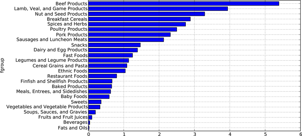
The tools that you need to slice and dice, aggregate, and visualize this dataset will be explored in detail in the next two chapters, so after you get a handle on those methods you might return to this dataset. For example, we could a plot of median values by food group and nutrient type (see Figure 7-1):
In [281]: result = ndata.groupby(['nutrient', 'fgroup'])['value'].quantile(0.5)

In [282]: result['Zinc, Zn'].order().plot(kind='barh')
With a little cleverness, you can find which food is most dense in each nutrient:
by_nutrient = ndata.groupby(['nutgroup', 'nutrient'])

get_maximum = lambda x: x.xs(x.value.idxmax())
get_minimum = lambda x: x.xs(x.value.idxmin())

max_foods = by_nutrient.apply(get_maximum)[['value', 'food']]

# make the food a little smaller
max_foods.food = max_foods.food.str[:50]
The resulting DataFrame is a bit too large to display in the book;
here is just the 'Amino Acids' nutrient
group:
In [284]: max_foods.ix['Amino Acids']['food']
Out[284]:
nutrient
Alanine          Gelatins, dry powder, unsweetened
Arginine              Seeds, sesame flour, low-fat
Aspartic acid                  Soy protein isolate
...
Tryptophan     Sea lion, Steller, meat with fat (Alaska Native)
Tyrosine      Soy protein isolate, PROTEIN TECHNOLOGIES INTE...
Valine        Soy protein isolate, PROTEIN TECHNOLOGIES INTE...
Name: food, Length: 19, dtype: object