
Time series data is an important form of structured data in many different fields, such as finance, economics, ecology, neuroscience, or physics. Anything that is observed or measured at many points in time forms a time series. Many time series are fixed frequency, which is to say that data points occur at regular intervals according to some rule, such as every 15 seconds, every 5 minutes, or once per month. Time series can also be irregular without a fixed unit or time or offset between units. How you mark and refer to time series data depends on the application and you may have one of the following:
Fixed periods, such as the month January 2007 or the full year 2010
Intervals of time, indicated by a start and end timestamp. Periods can be thought of as special cases of intervals
Experiment or elapsed time; each timestamp is a measure of time relative to a particular start time. For example, the diameter of a cookie baking each second since being placed in the oven
In this chapter, I am mainly concerned with time series in the first 3 categories, though many of the techniques can be applied to experimental time series where the index may be an integer or floating point number indicating elapsed time from the start of the experiment. The simplest and most widely used kind of time series are those indexed by timestamp.
pandas provides a standard set of time series tools and data algorithms. With this, you can efficiently work with very large time series and easily slice and dice, aggregate, and resample irregular and fixed frequency time series. As you might guess, many of these tools are especially useful for financial and economics applications, but you could certainly use them to analyze server log data, too.
Note
Some of the features and code, in particular period logic, presented
in this chapter were derived from the now defunct scikits.timeseries library.
The Python standard library includes data types for date and
time data, as well as calendar-related functionality. The datetime, time, and calendar modules are the
main places to start. The datetime.datetime type, or simply datetime, is widely used:
In [13]: from datetime import datetime

In [14]: now = datetime.now()

In [15]: now
Out[15]: datetime.datetime(2014, 7, 31, 0, 2, 55, 874995)

In [16]: now.year, now.month, now.day
Out[16]: (2014, 7, 31)
datetime stores both the date and
time down to the microsecond. datetime.timedelta represents the temporal
difference between two datetime
objects:
In [17]: delta = datetime(2011, 1, 7) - datetime(2008, 6, 24, 8, 15)

In [18]: delta
Out[18]: datetime.timedelta(926, 56700)

In [19]: delta.days        In [20]: delta.seconds
Out[19]: 926               Out[20]: 56700
You can add (or subtract) a timedelta or multiple thereof to a datetime object to yield a new shifted
object:
In [21]: from datetime import timedelta

In [22]: start = datetime(2011, 1, 7)

In [23]: start + timedelta(12)
Out[23]: datetime.datetime(2011, 1, 19, 0, 0)

In [24]: start - 2 * timedelta(12)
Out[24]: datetime.datetime(2010, 12, 14, 0, 0)
The data types in the datetime
module are summarized in Table 10-1. While
this chapter is mainly concerned with the data types in pandas and higher
level time series manipulation, you will undoubtedly encounter the
datetime-based types in many other
places in Python the wild.
datetime objects and
pandas Timestamp objects, which I’ll
introduce later, can be formatted as strings using str or the strftime method,
passing a format specification:
In [25]: stamp = datetime(2011, 1, 3)

In [26]: str(stamp)                   In [27]: stamp.strftime('%Y-%m-%d')
Out[26]: '2011-01-03 00:00:00'        Out[27]: '2011-01-03'
See Table 10-2 for a complete
list of the format codes. These same format codes can be used to convert
strings to dates using datetime.strptime:
In [28]: value = '2011-01-03'

In [29]: datetime.strptime(value, '%Y-%m-%d')
Out[29]: datetime.datetime(2011, 1, 3, 0, 0)

In [30]: datestrs = ['7/6/2011', '8/6/2011']

In [31]: [datetime.strptime(x, '%m/%d/%Y') for x in datestrs]
Out[31]: [datetime.datetime(2011, 7, 6, 0, 0), datetime.datetime(2011, 8, 6, 0, 0)]
datetime.strptime is
the best way to parse a date with a known format. However, it can be a
bit annoying to have to write a format spec each time, especially for
common date formats. In this case, you can use the parser.parse method in
the third party dateutil
package:
In [32]: from dateutil.parser import parse

In [33]: parse('2011-01-03')
Out[33]: datetime.datetime(2011, 1, 3, 0, 0)
dateutil is capable of parsing
almost any human-intelligible date representation:
In [34]: parse('Jan 31, 1997 10:45 PM')
Out[34]: datetime.datetime(1997, 1, 31, 22, 45)
In international locales, day appearing before month is very
common, so you can pass dayfirst=True
to indicate this:
In [35]: parse('6/12/2011', dayfirst=True)
Out[35]: datetime.datetime(2011, 12, 6, 0, 0)
pandas is generally oriented toward working with arrays of dates,
whether used as an axis index or a column in a DataFrame. The to_datetime method
parses many different kinds of date representations. Standard date
formats like ISO8601 can be parsed very quickly.
In [36]: datestrs
Out[36]: ['7/6/2011', '8/6/2011']

In [37]: pd.to_datetime(datestrs)
Out[37]:
<class 'pandas.tseries.index.DatetimeIndex'>
[2011-07-06, 2011-08-06]
Length: 2, Freq: None, Timezone: None
It also handles values that should be considered missing (None, empty string, etc.):
In [38]: idx = pd.to_datetime(datestrs + [None])

In [39]: idx
Out[39]:
<class 'pandas.tseries.index.DatetimeIndex'>
[2011-07-06, ..., NaT]
Length: 3, Freq: None, Timezone: None

In [40]: idx[2]
Out[40]: NaT

In [41]: pd.isnull(idx)
Out[41]: array([False, False,  True], dtype=bool)
NaT (Not a Time) is pandas’s NA
value for timestamp data.
Caution
dateutil.parser is a useful,
but not perfect tool. Notably, it will recognize some strings as dates
that you might prefer that it didn’t, like '42' will be parsed as the year 2042 with today’s calendar date.
Table 10-2. Datetime format specification (ISO C89 compatible)
datetime objects also have a
number of locale-specific formatting options for systems in other
countries or languages. For example, the abbreviated month names will be
different on German or French systems compared with English systems.
Table 10-3. Locale-specific date formatting
The most basic kind of time series object in pandas is a
Series indexed by timestamps, which is often represented external to
pandas as Python strings or datetime
objects:
In [42]: from datetime import datetime

In [43]: dates = [datetime(2011, 1, 2), datetime(2011, 1, 5), datetime(2011, 1, 7),
   ....:          datetime(2011, 1, 8), datetime(2011, 1, 10), datetime(2011, 1, 12)]

In [44]: ts = Series(np.random.randn(6), index=dates)

In [45]: ts
Out[45]:
2011-01-02   -0.204708
2011-01-05    0.478943
2011-01-07   -0.519439
2011-01-08   -0.555730
2011-01-10    1.965781
2011-01-12    1.393406
dtype: float64
Under the hood, these datetime
objects have been put in a DatetimeIndex:
In [47]: ts.index
Out[47]:
<class 'pandas.tseries.index.DatetimeIndex'>
[2011-01-02, ..., 2011-01-12]
Length: 6, Freq: None, Timezone: None
Note
It’s not necessary to use the TimeSeries constructor explicitly; when
creating a Series with a DatetimeIndex, pandas knows that the object is
a time series.
Like other Series, arithmetic operations between differently-indexed time series automatically align on the dates:
In [48]: ts + ts[::2]
Out[48]:
2011-01-02   -0.409415
2011-01-05         NaN
2011-01-07   -1.038877
2011-01-08         NaN
2011-01-10    3.931561
2011-01-12         NaN
dtype: float64
pandas stores timestamps using NumPy’s datetime64 data type at the nanosecond
resolution:
In [49]: ts.index.dtype
Out[49]: dtype('<M8[ns]')
Scalar values from a DatetimeIndex are pandas Timestamp objects
In [50]: stamp = ts.index[0]

In [51]: stamp
Out[51]: Timestamp('2011-01-02 00:00:00')
A Timestamp can be substituted
anywhere you would use a datetime
object. Additionally, it can store frequency information (if any) and
understands how to do time zone conversions and other kinds of
manipulations. More on both of these things later.
TimeSeries is a subclass of Series and thus behaves in the same way with regard to indexing and selecting data based on label:
In [52]: stamp = ts.index[2]

In [53]: ts[stamp]
Out[53]: -0.51943871505673822
As a convenience, you can also pass a string that is interpretable as a date:
In [54]: ts['1/10/2011']           In [55]: ts['20110110']
Out[54]: 1.9657805725027142        Out[55]: 1.9657805725027142
For longer time series, a year or only a year and month can be passed to easily select slices of data:
In [56]: longer_ts = Series(np.random.randn(1000),
   ....:                    index=pd.date_range('1/1/2000', periods=1000))

In [57]: longer_ts
Out[57]:
2000-01-01    0.092908
2000-01-02    0.281746
2000-01-03    0.769023
2000-01-04    1.246435
...
2002-09-23   -0.811676
2002-09-24   -1.830156
2002-09-25   -0.138730
2002-09-26    0.334088
Freq: D, Length: 1000

In [58]: longer_ts['2001']        In [59]: longer_ts['2001-05']
Out[58]:                          Out[59]:
2001-01-01    1.599534            2001-05-01   -0.622547
2001-01-02    0.474071            2001-05-02    0.936289
2001-01-03    0.151326            2001-05-03    0.750018
2001-01-04   -0.542173            2001-05-04   -0.056715
...                               ...
2001-12-28   -0.433739            2001-05-28    0.111835
2001-12-29    0.092698            2001-05-29   -1.251504
2001-12-30   -1.397820            2001-05-30   -2.949343
2001-12-31    1.457823            2001-05-31    0.634634
Freq: D, Length: 365              Freq: D, Length: 31
Slicing with dates works just like with a regular Series:
In [60]: ts[datetime(2011, 1, 7):]
Out[60]:
2011-01-07   -0.519439
2011-01-08   -0.555730
2011-01-10    1.965781
2011-01-12    1.393406
dtype: float64
Because most time series data is ordered chronologically, you can slice with timestamps not contained in a time series to perform a range query:
In [61]: ts                   In [62]: ts['1/6/2011':'1/11/2011']
Out[61]:                      Out[62]:
2011-01-02   -0.204708        2011-01-07   -0.519439
2011-01-05    0.478943        2011-01-08   -0.555730
2011-01-07   -0.519439        2011-01-10    1.965781
2011-01-08   -0.555730        dtype: float64
2011-01-10    1.965781
2011-01-12    1.393406
dtype: float64
As before you can pass either a string date, datetime, or
Timestamp. Remember that slicing in this manner produces views on the
source time series just like slicing NumPy arrays. There is an
equivalent instance method truncate which slices a
TimeSeries between two dates:
In [63]: ts.truncate(after='1/9/2011')
Out[63]:
2011-01-02   -0.204708
2011-01-05    0.478943
2011-01-07   -0.519439
2011-01-08   -0.555730
dtype: float64
All of the above holds true for DataFrame as well, indexing on its rows:
In [64]: dates = pd.date_range('1/1/2000', periods=100, freq='W-WED')

In [65]: long_df = DataFrame(np.random.randn(100, 4),
   ....:                     index=dates,
   ....:                     columns=['Colorado', 'Texas', 'New York', 'Ohio'])

In [66]: long_df.ix['5-2001']
Out[66]:
            Colorado     Texas  New York      Ohio
2001-05-02 -0.006045  0.490094 -0.277186 -0.707213
2001-05-09 -0.560107  2.735527  0.927335  1.513906
2001-05-16  0.538600  1.273768  0.667876 -0.969206
2001-05-23  1.676091 -0.817649  0.050188  1.951312
2001-05-30 3.260383 0.963301 1.201206 -1.852001In some applications, there may be multiple data observations falling on a particular timestamp. Here is an example:
In [67]: dates = pd.DatetimeIndex(['1/1/2000', '1/2/2000', '1/2/2000', '1/2/2000',
   ....:                           '1/3/2000'])

In [68]: dup_ts = Series(np.arange(5), index=dates)

In [69]: dup_ts
Out[69]:
2000-01-01    0
2000-01-02    1
2000-01-02    2
2000-01-02    3
2000-01-03    4
dtype: int64
We can tell that the index is not unique by checking its is_unique property:
In [70]: dup_ts.index.is_unique
Out[70]: False
Indexing into this time series will now either produce scalar values or slices depending on whether a timestamp is duplicated:
In [71]: dup_ts['1/3/2000']  # not duplicated
Out[71]: 4

In [72]: dup_ts['1/2/2000']  # duplicated
Out[72]:
2000-01-02    1
2000-01-02    2
2000-01-02    3
dtype: int64
Suppose you wanted to aggregate the data having non-unique
timestamps. One way to do this is to use groupby and pass
level=0 (the only level of
indexing!):
In [73]: grouped = dup_ts.groupby(level=0)

In [74]: grouped.mean()      In [75]: grouped.count()
Out[74]:                     Out[75]:
2000-01-01    0              2000-01-01    1
2000-01-02    2              2000-01-02    3
2000-01-03    4              2000-01-03    1
dtype: int64                 dtype: int64
Generic time series in pandas are assumed to be irregular; that is,
they have no fixed frequency. For many applications this is sufficient.
However, it’s often desirable to work relative to a fixed frequency, such
as daily, monthly, or every 15 minutes, even if that means introducing
missing values into a time series. Fortunately pandas has a full suite of
standard time series frequencies and tools for resampling, inferring
frequencies, and generating fixed frequency date ranges. For example, in
the example time series, converting it to be fixed daily frequency can be
accomplished by calling resample:
In [76]: ts                   In [77]: ts.resample('D')
Out[76]:                      Out[77]:
2011-01-02   -0.204708        2011-01-02   -0.204708
2011-01-05    0.478943        2011-01-03         NaN
2011-01-07   -0.519439        2011-01-04         NaN
2011-01-08   -0.555730        2011-01-05    0.478943
2011-01-10    1.965781        2011-01-06         NaN
2011-01-12    1.393406        2011-01-07   -0.519439
dtype: float64                2011-01-08   -0.555730
                              2011-01-09         NaN
                              2011-01-10    1.965781
                              2011-01-11         NaN
                              2011-01-12    1.393406
                              Freq: D, dtype: float64
Conversion between frequencies or resampling is a big enough topic to have its own section later. Here I’ll show you how to use the base frequencies and multiples thereof.
While I used it previously without explanation, you may
have guessed that pandas.date_range is
responsible for generating a DatetimeIndex with an indicated length
according to a particular frequency:
In [78]: index = pd.date_range('4/1/2012', '6/1/2012')

In [79]: index
Out[79]:
<class 'pandas.tseries.index.DatetimeIndex'>
[2012-04-01, ..., 2012-06-01]
Length: 62, Freq: D, Timezone: None
By default, date_range generates
daily timestamps. If you pass only a start or end date, you must pass a
number of periods to generate:
In [80]: pd.date_range(start='4/1/2012', periods=20)
Out[80]:
<class 'pandas.tseries.index.DatetimeIndex'>
[2012-04-01, ..., 2012-04-20]
Length: 20, Freq: D, Timezone: None

In [81]: pd.date_range(end='6/1/2012', periods=20)
Out[81]:
<class 'pandas.tseries.index.DatetimeIndex'>
[2012-05-13, ..., 2012-06-01]
Length: 20, Freq: D, Timezone: None
The start and end dates define strict boundaries for the generated
date index. For example, if you wanted a date index containing the last
business day of each month, you would pass the 'BM' frequency (business end of month) and
only dates falling on or inside the date interval will be
included:
In [82]: pd.date_range('1/1/2000', '12/1/2000', freq='BM')
Out[82]:
<class 'pandas.tseries.index.DatetimeIndex'>
[2000-01-31, ..., 2000-11-30]
Length: 11, Freq: BM, Timezone: None
date_range by default
preserves the time (if any) of the start or end timestamp:
In [83]: pd.date_range('5/2/2012 12:56:31', periods=5)
Out[83]:
<class 'pandas.tseries.index.DatetimeIndex'>
[2012-05-02 12:56:31, ..., 2012-05-06 12:56:31]
Length: 5, Freq: D, Timezone: None
Sometimes you will have start or end dates with time information
but want to generate a set of timestamps normalized to midnight as a
convention. To do this, there is a normalize option:
In [84]: pd.date_range('5/2/2012 12:56:31', periods=5, normalize=True)
Out[84]:
<class 'pandas.tseries.index.DatetimeIndex'>
[2012-05-02, ..., 2012-05-06]
Length: 5, Freq: D, Timezone: None
Frequencies in pandas are composed of a base
frequency and a multiplier. Base frequencies are typically
referred to by a string alias, like 'M' for monthly or 'H' for hourly. For each base frequency, there
is an object defined generally referred to as a date
offset. For example, hourly frequency can be represented with
the Hour class:
In [85]: from pandas.tseries.offsets import Hour, Minute

In [86]: hour = Hour()

In [87]: hour
Out[87]: <Hour>
You can define a multiple of an offset by passing an integer:
In [88]: four_hours = Hour(4)

In [89]: four_hours
Out[89]: <4 * Hours>
In most applications, you would never need to explicitly create
one of these objects, instead using a string alias like 'H' or '4H'. Putting an integer before the base
frequency creates a multiple:
In [90]: pd.date_range('1/1/2000', '1/3/2000 23:59', freq='4h')
Out[90]:
<class 'pandas.tseries.index.DatetimeIndex'>
[2000-01-01 00:00:00, ..., 2000-01-03 20:00:00]
Length: 18, Freq: 4H, Timezone: None
Many offsets can be combined together by addition:
In [91]: Hour(2) + Minute(30)
Out[91]: <150 * Minutes>
Similarly, you can pass frequency strings like '2h30min' which will effectively be parsed to
the same expression:
In [92]: pd.date_range('1/1/2000', periods=10, freq='1h30min')
Out[92]:
<class 'pandas.tseries.index.DatetimeIndex'>
[2000-01-01 00:00:00, ..., 2000-01-01 13:30:00]
Length: 10, Freq: 90T, Timezone: None
Some frequencies describe points in time that are not evenly
spaced. For example, 'M' (calendar
month end) and 'BM' (last
business/weekday of month) depend on the number of days in a month and,
in the latter case, whether the month ends on a weekend or not. For lack
of a better term, I call these anchored
offsets.
See Table 10-4 for a listing of frequency codes and date offset classes available in pandas.
Note
Users can define their own custom frequency classes to provide date logic not available in pandas, though the full details of that are outside the scope of this book.
Table 10-4. Base Time Series Frequencies
| Alias | Offset Type | Description |
|---|---|---|
| D | Day | Calendar daily |
| B | BusinessDay | Business daily |
| H | Hour | Hourly |
| T or min | Minute | Minutely |
| S | Second | Secondly |
| L or ms | Milli | Millisecond (1/1000th of 1 second) |
| U | Micro | Microsecond (1/1000000th of 1 second) |
| M | MonthEnd | Last calendar day of month |
| BM | BusinessMonthEnd | Last business day (weekday) of month |
| MS | MonthBegin | First calendar day of month |
| BMS | BusinessMonthBegin | First weekday of month |
W-MON, W-TUE,
... | Week | Weekly on given day of week: MON, TUE, WED, THU, FRI, SAT, or SUN. |
WOM-1MON, WOM-2MON,
... | WeekOfMonth | Generate weekly dates in the first, second, third, or
fourth week of the month. For example, WOM-3FRI for the 3rd Friday of each
month. |
Q-JAN, Q-FEB,
... | QuarterEnd | Quarterly dates anchored on last calendar day of each month, for year ending in indicated month: JAN, FEB, MAR, APR, MAY, JUN, JUL, AUG, SEP, OCT, NOV, or DEC. |
BQ-JAN, BQ-FEB,
... | BusinessQuarterEnd | Quarterly dates anchored on last weekday day of each month, for year ending in indicated month |
QS-JAN, QS-FEB,
... | QuarterBegin | Quarterly dates anchored on first calendar day of each month, for year ending in indicated month |
BQS-JAN, BQS-FEB,
... | BusinessQuarterBegin | Quarterly dates anchored on first weekday day of each month, for year ending in indicated month |
A-JAN, A-FEB,
... | YearEnd | Annual dates anchored on last calendar day of given month: JAN, FEB, MAR, APR, MAY, JUN, JUL, AUG, SEP, OCT, NOV, or DEC. |
BA-JAN, BA-FEB,
... | BusinessYearEnd | Annual dates anchored on last weekday of given month |
AS-JAN, AS-FEB,
... | YearBegin | Annual dates anchored on first day of given month |
BAS-JAN, BAS-FEB,
... | BusinessYearBegin | Annual dates anchored on first weekday of given month |
One useful frequency class is “week of month”, starting
with WOM. This enables you to get
dates like the third Friday of each month:
In [93]: rng = pd.date_range('1/1/2012', '9/1/2012', freq='WOM-3FRI')

In [94]: list(rng)
Out[94]:
[Timestamp('2012-01-20 00:00:00', offset='WOM-3FRI'),
 Timestamp('2012-02-17 00:00:00', offset='WOM-3FRI'),
 Timestamp('2012-03-16 00:00:00', offset='WOM-3FRI'),
 Timestamp('2012-04-20 00:00:00', offset='WOM-3FRI'),
 Timestamp('2012-05-18 00:00:00', offset='WOM-3FRI'),
 Timestamp('2012-06-15 00:00:00', offset='WOM-3FRI'),
 Timestamp('2012-07-20 00:00:00', offset='WOM-3FRI'),
 Timestamp('2012-08-17 00:00:00', offset='WOM-3FRI')]
Traders of US equity options will recognize these dates as the standard dates of monthly expiry.
“Shifting” refers to moving data backward and forward
through time. Both Series and DataFrame have a shift method for doing naive shifts forward or
backward, leaving the index unmodified:
In [95]: ts = Series(np.random.randn(4),
   ....:             index=pd.date_range('1/1/2000', periods=4, freq='M'))

In [96]: ts                  In [97]: ts.shift(2)         In [98]: ts.shift(-2)
Out[96]:                     Out[97]:                     Out[98]:
2000-01-31   -0.066748       2000-01-31         NaN       2000-01-31   -0.117388
2000-02-29    0.838639       2000-02-29         NaN       2000-02-29   -0.517795
2000-03-31   -0.117388       2000-03-31   -0.066748       2000-03-31         NaN
2000-04-30   -0.517795       2000-04-30    0.838639       2000-04-30         NaN
Freq: M, dtype: float64      Freq: M, dtype: float64      Freq: M, dtype: float64
A common use of shift is
computing percent changes in a time series or multiple time series as
DataFrame columns. This is expressed as
ts / ts.shift(1) - 1
Because naive shifts leave the index unmodified, some data is
discarded. Thus if the frequency is known, it can be passed to shift to advance the timestamps instead of
simply the data:
In [99]: ts.shift(2, freq='M')
Out[99]:
2000-03-31   -0.066748
2000-04-30    0.838639
2000-05-31   -0.117388
2000-06-30   -0.517795
Freq: M, dtype: float64
Other frequencies can be passed, too, giving you a lot of flexibility in how to lead and lag the data:
In [100]: ts.shift(3, freq='D')        In [101]: ts.shift(1, freq='3D')
Out[100]:                              Out[101]:
2000-02-03   -0.066748                 2000-02-03   -0.066748
2000-03-03    0.838639                 2000-03-03    0.838639
2000-04-03   -0.117388                 2000-04-03   -0.117388
2000-05-03   -0.517795                 2000-05-03   -0.517795
dtype: float64                         dtype: float64

In [102]: ts.shift(1, freq='90T')
Out[102]:
2000-01-31 01:30:00   -0.066748
2000-02-29 01:30:00    0.838639
2000-03-31 01:30:00   -0.117388
2000-04-30 01:30:00   -0.517795
dtype: float64
The pandas date offsets can also be used with datetime or Timestamp objects:
In [103]: from pandas.tseries.offsets import Day, MonthEnd

In [104]: now = datetime(2011, 11, 17)

In [105]: now + 3 * Day()
Out[105]: Timestamp('2011-11-20 00:00:00')
If you add an anchored offset like MonthEnd, the first increment will roll forward a date to the next date
according to the frequency rule:
In [106]: now + MonthEnd()
Out[106]: Timestamp('2011-11-30 00:00:00')

In [107]: now + MonthEnd(2)
Out[107]: Timestamp('2011-12-31 00:00:00')
Anchored offsets can explicitly “roll” dates forward or backward
using their rollforward and
rollback methods,
respectively:
In [108]: offset = MonthEnd()

In [109]: offset.rollforward(now)
Out[109]: Timestamp('2011-11-30 00:00:00')

In [110]: offset.rollback(now)
Out[110]: Timestamp('2011-10-31 00:00:00')
A clever use of date offsets is to use these methods with
groupby:
In [111]: ts = Series(np.random.randn(20),
   .....:             index=pd.date_range('1/15/2000', periods=20, freq='4d'))

In [112]: ts.groupby(offset.rollforward).mean()
Out[112]:
2000-01-31   -0.005833
2000-02-29    0.015894
2000-03-31    0.150209
dtype: float64
Of course, an easier and faster way to do this is using resample (much more on this
later):
In [113]: ts.resample('M', how='mean')
Out[113]:
2000-01-31   -0.005833
2000-02-29    0.015894
2000-03-31    0.150209
Freq: M, dtype: float64Working with time zones is generally considered one of the most unpleasant parts of time series manipulation. In particular, daylight savings time (DST) transitions are a common source of complication. As such, many time series users choose to work with time series in coordinated universal time or UTC, which is the successor to Greenwich Mean Time and is the current international standard. Time zones are expressed as offsets from UTC; for example, New York is four hours behind UTC during daylight savings time and 5 hours the rest of the year.
In Python, time zone information comes from the 3rd party pytz library, which
exposes the Olson database, a compilation of world
time zone information. This is especially important for historical data
because the DST transition dates (and even UTC offsets) have been changed
numerous times depending on the whims of local governments. In the United
States,the DST transition times have been changed many times since
1900!
For detailed information about pytz library, you’ll need
to look at that library’s documentation. As far as this book is concerned,
pandas wraps pytz’s functionality so
you can ignore its API outside of the time zone names. Time zone names can
be found interactively and in the docs:
In [114]: import pytz

In [115]: pytz.common_timezones[-5:]
Out[115]: ['US/Eastern', 'US/Hawaii', 'US/Mountain', 'US/Pacific', 'UTC']
To get a time zone object from pytz, use pytz.timezone:
In [116]: tz = pytz.timezone('US/Eastern')

In [117]: tz
Out[117]: <DstTzInfo 'US/Eastern' LMT-1 day, 19:04:00 STD>
Methods in pandas will accept either time zone names or these objects. I recommend just using the names.
By default, time series in pandas are time zone naive. Consider the following time series:
rng = pd.date_range('3/9/2012 9:30', periods=6, freq='D')
ts = Series(np.random.randn(len(rng)), index=rng)
The index’s tz field is
None:
In [119]: print(ts.index.tz)
None
Date ranges can be generated with a time zone set:
In [120]: pd.date_range('3/9/2012 9:30', periods=10, freq='D', tz='UTC')
Out[120]:
<class 'pandas.tseries.index.DatetimeIndex'>
[2012-03-09 09:30:00+00:00, ..., 2012-03-18 09:30:00+00:00]
Length: 10, Freq: D, Timezone: UTC
Conversion from naive to localized is handled
by the tz_localize
method:
In [121]: ts_utc = ts.tz_localize('UTC')

In [122]: ts_utc
Out[122]:
2012-03-09 09:30:00+00:00   -0.202469
2012-03-10 09:30:00+00:00    0.050718
2012-03-11 09:30:00+00:00    0.639869
2012-03-12 09:30:00+00:00    0.597594
2012-03-13 09:30:00+00:00   -0.797246
2012-03-14 09:30:00+00:00    0.472879
Freq: D, dtype: float64

In [123]: ts_utc.index
Out[123]:
<class 'pandas.tseries.index.DatetimeIndex'>
[2012-03-09 09:30:00+00:00, ..., 2012-03-14 09:30:00+00:00]
Length: 6, Freq: D, Timezone: UTC
Once a time series has been localized to a particular time zone,
it can be converted to another time zone using tz_convert:
In [124]: ts_utc.tz_convert('US/Eastern')
Out[124]:
2012-03-09 04:30:00-05:00   -0.202469
2012-03-10 04:30:00-05:00    0.050718
2012-03-11 05:30:00-04:00    0.639869
2012-03-12 05:30:00-04:00    0.597594
2012-03-13 05:30:00-04:00   -0.797246
2012-03-14 05:30:00-04:00    0.472879
Freq: D, dtype: float64
In the case of the above time series, which straddles a DST transition in the US/Eastern time zone, we could localize to EST and convert to, say, UTC or Berlin time:
In [125]: ts_eastern = ts.tz_localize('US/Eastern')

In [126]: ts_eastern.tz_convert('UTC')
Out[126]:
2012-03-09 14:30:00+00:00   -0.202469
2012-03-10 14:30:00+00:00    0.050718
2012-03-11 13:30:00+00:00    0.639869
2012-03-12 13:30:00+00:00    0.597594
2012-03-13 13:30:00+00:00   -0.797246
2012-03-14 13:30:00+00:00    0.472879
Freq: D, dtype: float64

In [127]: ts_eastern.tz_convert('Europe/Berlin')
Out[127]:
2012-03-09 15:30:00+01:00   -0.202469
2012-03-10 15:30:00+01:00    0.050718
2012-03-11 14:30:00+01:00    0.639869
2012-03-12 14:30:00+01:00    0.597594
2012-03-13 14:30:00+01:00   -0.797246
2012-03-14 14:30:00+01:00    0.472879
Freq: D, dtype: float64
tz_localize and
tz_convert are also
instance methods on DatetimeIndex:
In [128]: ts.index.tz_localize('Asia/Shanghai')
Out[128]:
<class 'pandas.tseries.index.DatetimeIndex'>
[2012-03-09 09:30:00+08:00, ..., 2012-03-14 09:30:00+08:00]
Length: 6, Freq: D, Timezone: Asia/ShanghaiSimilar to time series and date ranges, individual Timestamp objects similarly can be localized from naive to time zone-aware and converted from one time zone to another:
In [129]: stamp = pd.Timestamp('2011-03-12 04:00')

In [130]: stamp_utc = stamp.tz_localize('utc')

In [131]: stamp_utc.tz_convert('US/Eastern')
Out[131]: Timestamp('2011-03-11 23:00:00-0500', tz='US/Eastern')
You can also pass a time zone when creating the Timestamp:
In [132]: stamp_moscow = pd.Timestamp('2011-03-12 04:00', tz='Europe/Moscow')

In [133]: stamp_moscow
Out[133]: Timestamp('2011-03-12 04:00:00+0300', tz='Europe/Moscow')
Time zone-aware Timestamp objects internally store a UTC timestamp value as nanoseconds since the UNIX epoch (January 1, 1970); this UTC value is invariant between time zone conversions:
In [134]: stamp_utc.value
Out[134]: 1299902400000000000

In [135]: stamp_utc.tz_convert('US/Eastern').value
Out[135]: 1299902400000000000
When performing time arithmetic using pandas’s DateOffset objects, daylight savings time
transitions are respected where possible:
# 30 minutes before DST transition
from pandas.tseries.offsets import Hour
stamp = pd.Timestamp('2012-03-12 01:30', tz='US/Eastern')
stamp
stamp + Hour()

# 90 minutes before DST transition
stamp = pd.Timestamp('2012-11-04 00:30', tz='US/Eastern')
stamp
stamp + 2 * Hour()If two time series with different time zones are combined, the result will be UTC. Since the timestamps are stored under the hood in UTC, this is a straightforward operation and requires no conversion to happen:
In [140]: rng = pd.date_range('3/7/2012 9:30', periods=10, freq='B')

In [141]: ts = Series(np.random.randn(len(rng)), index=rng)

In [142]: ts
Out[142]:
2012-03-07 09:30:00    0.522356
2012-03-08 09:30:00   -0.546348
2012-03-09 09:30:00   -0.733537
2012-03-12 09:30:00    1.302736
2012-03-13 09:30:00    0.022199
2012-03-14 09:30:00    0.364287
2012-03-15 09:30:00   -0.922839
2012-03-16 09:30:00    0.312656
2012-03-19 09:30:00   -1.128497
2012-03-20 09:30:00   -0.333488
Freq: B, dtype: float64

In [143]: ts1 = ts[:7].tz_localize('Europe/London')

In [144]: ts2 = ts1[2:].tz_convert('Europe/Moscow')

In [145]: result = ts1 + ts2

In [146]: result.index
Out[146]:
<class 'pandas.tseries.index.DatetimeIndex'>
[2012-03-07 09:30:00+00:00, ..., 2012-03-15 09:30:00+00:00]
Length: 7, Freq: B, Timezone: UTC
Periods represent time spans, like
days, months, quarters, or years. The Period class represents
this data type, requiring a string or integer and a frequency from the
above table:
In [147]: p = pd.Period(2007, freq='A-DEC')

In [148]: p
Out[148]: Period('2007', 'A-DEC')
In this case, the Period object
represents the full timespan from January 1, 2007 to December 31, 2007,
inclusive. Conveniently, adding and subtracting integers from periods has
the effect of shifting by their frequency:
In [149]: p + 5                          In [150]: p - 2
Out[149]: Period('2012', 'A-DEC')        Out[150]: Period('2005', 'A-DEC')
If two periods have the same frequency, their difference is the number of units between them:
In [151]: pd.Period('2014', freq='A-DEC') - p
Out[151]: 7
Regular ranges of periods can be constructed using the period_range
function:
In [152]: rng = pd.period_range('1/1/2000', '6/30/2000', freq='M')

In [153]: rng
Out[153]:
<class 'pandas.tseries.period.PeriodIndex'>
[2000-01, ..., 2000-06]
Length: 6, Freq: M
The PeriodIndex class stores a
sequence of periods and can serve as an axis index in any pandas data
structure:
In [154]: Series(np.random.randn(6), index=rng)
Out[154]:
2000-01   -0.514551
2000-02   -0.559782
2000-03   -0.783408
2000-04   -1.797685
2000-05   -0.172670
2000-06    0.680215
Freq: M, dtype: float64
If you have an array of strings, you can also appeal to the PeriodIndex class itself:
In [155]: values = ['2001Q3', '2002Q2', '2003Q1']

In [156]: index = pd.PeriodIndex(values, freq='Q-DEC')

In [157]: index
Out[157]:
<class 'pandas.tseries.period.PeriodIndex'>
[2001Q3, ..., 2003Q1]
Length: 3, Freq: Q-DEC
Periods and PeriodIndex
objects can be converted to another frequency using their asfreq method. As an
example, suppose we had an annual period and wanted to convert it into a
monthly period either at the start or end of the year. This is fairly
straightforward:
In [158]: p = pd.Period('2007', freq='A-DEC')

In [159]: p.asfreq('M', how='start')      In [160]: p.asfreq('M', how='end')
Out[159]: Period('2007-01', 'M')          Out[160]: Period('2007-12', 'M')
You can think of Period('2007',
'A-DEC') as being a cursor pointing to a span of time,
subdivided by monthly periods. See Figure 10-1 for an illustration of this. For a
fiscal year ending on a month other than December,
the monthly subperiods belonging are different:
In [161]: p = pd.Period('2007', freq='A-JUN')

In [162]: p.asfreq('M', 'start')      In [163]: p.asfreq('M', 'end')
Out[162]: Period('2006-07', 'M')      Out[163]: Period('2007-06', 'M')
When converting from high to low frequency, the superperiod will
be determined depending on where the subperiod “belongs”. For example,
in A-JUN frequency, the month
Aug-2007 is actually part of the
2008 period:
In [164]: p = pd.Period('Aug-2007', 'M')

In [165]: p.asfreq('A-JUN')
Out[165]: Period('2008', 'A-JUN')
Whole PeriodIndex objects or
TimeSeries can be similarly converted with the same semantics:
In [166]: rng = pd.period_range('2006', '2009', freq='A-DEC')

In [167]: ts = Series(np.random.randn(len(rng)), index=rng)

In [168]: ts
Out[168]:
2006    1.607578
2007    0.200381
2008   -0.834068
2009   -0.302988
Freq: A-DEC, dtype: float64

In [169]: ts.asfreq('M', how='start')      In [170]: ts.asfreq('B', how='end')
Out[169]:                                  Out[170]:
2006-01    1.607578                        2006-12-29    1.607578
2007-01    0.200381                        2007-12-31    0.200381
2008-01   -0.834068                        2008-12-31   -0.834068
2009-01   -0.302988                        2009-12-31   -0.302988
Freq: M, dtype: float64                    Freq: B, dtype: float64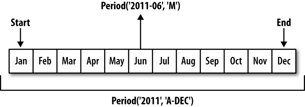
Quarterly data is standard in accounting, finance, and
other fields. Much quarterly data is reported relative to a
fiscal year end, typically the last calendar or
business day of one of the 12 months of the year. As such, the period
2012Q4 has a different meaning
depending on fiscal year end. pandas supports all 12 possible quarterly
frequencies as Q-JAN through Q-DEC:
In [171]: p = pd.Period('2012Q4', freq='Q-JAN')

In [172]: p
Out[172]: Period('2012Q4', 'Q-JAN')
In the case of fiscal year ending in January, 2012Q4 runs from November through January,
which you can check by converting to daily frequency. See Figure 10-2 for an illustration:
In [173]: p.asfreq('D', 'start')         In [174]: p.asfreq('D', 'end')
Out[173]: Period('2011-11-01', 'D')      Out[174]: Period('2012-01-31', 'D')
Thus, it’s possible to do period arithmetic very easily; for example, to get the timestamp at 4PM on the 2nd to last business day of the quarter, you could do:
In [175]: p4pm = (p.asfreq('B', 'e') - 1).asfreq('T', 's') + 16 * 60

In [176]: p4pm
Out[176]: Period('2012-01-30 16:00', 'T')

In [177]: p4pm.to_timestamp()
Out[177]: Timestamp('2012-01-30 16:00:00')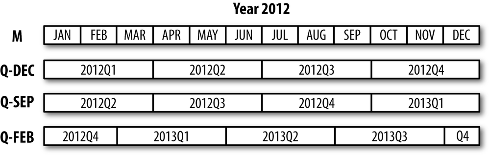
Generating quarterly ranges works as you would expect using
period_range.
Arithmetic is identical, too:
In [178]: rng = pd.period_range('2011Q3', '2012Q4', freq='Q-JAN')

In [179]: ts = Series(np.arange(len(rng)), index=rng)

In [180]: ts
Out[180]:
2011Q3    0
2011Q4    1
2012Q1    2
2012Q2    3
2012Q3    4
2012Q4    5
Freq: Q-JAN, dtype: int64

In [181]: new_rng = (rng.asfreq('B', 'e') - 1).asfreq('T', 's') + 16 * 60

In [182]: ts.index = new_rng.to_timestamp()

In [183]: ts
Out[183]:
2010-10-28 16:00:00    0
2011-01-28 16:00:00    1
2011-04-28 16:00:00    2
2011-07-28 16:00:00    3
2011-10-28 16:00:00    4
2012-01-30 16:00:00    5
dtype: int64Series and DataFrame objects indexed by timestamps can be
converted to periods using the to_period
method:
In [184]: rng = pd.date_range('1/1/2000', periods=3, freq='M')

In [185]: ts = Series(randn(3), index=rng)

In [186]: pts = ts.to_period()

In [187]: ts                   In [188]: pts
Out[187]:                      Out[188]:
2000-01-31    1.663261         2000-01    1.663261
2000-02-29   -0.996206         2000-02   -0.996206
2000-03-31    1.521760         2000-03    1.521760
Freq: M, dtype: float64        Freq: M, dtype: float64
Since periods always refer to non-overlapping timespans, a
timestamp can only belong to a single period for a given frequency.
While the frequency of the new PeriodIndex is inferred
from the timestamps by default, you can specify any frequency you want.
There is also no problem with having duplicate periods in the
result:
In [189]: rng = pd.date_range('1/29/2000', periods=6, freq='D')

In [190]: ts2 = Series(randn(6), index=rng)

In [191]: ts2.to_period('M')
Out[191]:
2000-01    0.244175
2000-01    0.423331
2000-01   -0.654040
2000-02    2.089154
2000-02   -0.060220
2000-02   -0.167933
Freq: M, dtype: float64
To convert back to timestamps, use to_timestamp:
In [192]: pts = ts.to_period()

In [193]: pts
Out[193]:
2000-01    1.663261
2000-02   -0.996206
2000-03    1.521760
Freq: M, dtype: float64

In [194]: pts.to_timestamp(how='end')
Out[194]:
2000-01-31    1.663261
2000-02-29   -0.996206
2000-03-31    1.521760
Freq: M, dtype: float64
Fixed frequency data sets are sometimes stored with timespan information spread across multiple columns. For example, in this macroeconomic data set, the year and quarter are in different columns:
In [195]: data = pd.read_csv('ch08/macrodata.csv')

In [196]: data.year                            In [197]: data.quarter
Out[196]:                                      Out[197]:
0    1959                                      0    1
1    1959                                      1    2
2    1959                                      2    3
3    1959                                      3    4
...                                            ...
199    2008                                    199    4
200    2009                                    200    1
201    2009                                    201    2
202    2009                                    202    3
Name: year, Length: 203, dtype: float64        Name: quarter, Length: 203, dtype: float64
By passing these arrays to PeriodIndex with a
frequency, they can be combined to form an index for the
DataFrame:
In [198]: index = pd.PeriodIndex(year=data.year, quarter=data.quarter, freq='Q-DEC')

In [199]: index
Out[199]:
<class 'pandas.tseries.period.PeriodIndex'>
[1959Q1, ..., 2009Q3]
Length: 203, Freq: Q-DEC

In [200]: data.index = index

In [201]: data.infl
Out[201]:
1959Q1    0.00
1959Q2    2.34
1959Q3    2.74
1959Q4    0.27
...
2008Q4   -8.79
2009Q1    0.94
2009Q2    3.37
2009Q3    3.56
Freq: Q-DEC, Name: infl, Length: 203
Resampling refers to the process of
converting a time series from one frequency to another. Aggregating higher
frequency data to lower frequency is called downsampling, while converting lower
frequency to higher frequency is called upsampling. Not all resampling falls
into either of these categories; for example, converting W-WED (weekly on Wednesday) to W-FRI is neither upsampling nor
downsampling.
pandas objects are equipped with a resample method, which is the workhorse function
for all frequency conversion:
In [202]: rng = pd.date_range('1/1/2000', periods=100, freq='D')

In [203]: ts = Series(randn(len(rng)), index=rng)

In [204]: ts.resample('M', how='mean')
Out[204]:
2000-01-31   -0.165893
2000-02-29    0.078606
2000-03-31    0.223811
2000-04-30   -0.063643
Freq: M, dtype: float64

In [205]: ts.resample('M', how='mean', kind='period')
Out[205]:
2000-01   -0.165893
2000-02    0.078606
2000-03    0.223811
2000-04   -0.063643
Freq: M, dtype: float64
resample is a flexible and
high-performance method that can be used to process very large time
series. I’ll illustrate its semantics and use through a series of
examples.
Table 10-5. Resample method arguments
Aggregating data to a regular, lower frequency is a pretty
normal time series task. The data you’re aggregating doesn’t need to be
fixed frequently; the desired frequency defines bin
edges that are used to slice the time series into pieces to
aggregate. For example, to convert to monthly, 'M' or 'BM', the data need to be chopped up into one
month intervals. Each interval is said to be half-open; a data point can only
belong to one interval, and the union of the intervals must make up the
whole time frame. There are a couple things to think about when using
resample to downsample data:
Which side of each interval is closed
How to label each aggregated bin, either with the start of the interval or the end
To illustrate, let’s look at some one-minute data:
In [206]: rng = pd.date_range('1/1/2000', periods=12, freq='T')

In [207]: ts = Series(np.arange(12), index=rng)

In [208]: ts
Out[208]:
2000-01-01 00:00:00     0
2000-01-01 00:01:00     1
2000-01-01 00:02:00     2
2000-01-01 00:03:00     3
2000-01-01 00:04:00     4
2000-01-01 00:05:00     5
2000-01-01 00:06:00     6
2000-01-01 00:07:00     7
2000-01-01 00:08:00     8
2000-01-01 00:09:00     9
2000-01-01 00:10:00    10
2000-01-01 00:11:00    11
Freq: T, dtype: int64
Suppose you wanted to aggregate this data into five-minute chunks or bars by taking the sum of each group:
In [209]: ts.resample('5min', how='sum')
Out[209]:
2000-01-01 00:00:00 10
2000-01-01 00:05:00 35
2000-01-01 00:10:00 21
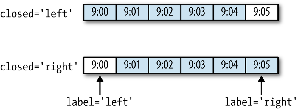
Freq: 5T, dtype: int64The frequency you pass defines bin edges in five-minute
increments. By default, the left bin edge is
inclusive, so the 00:00 value is
included in the 00:00 to 00:05 interval.[5] Passing closed='right'
changes the interval to be closed on the right:
In [210]: ts.resample('5min', how='sum', closed='right')
Out[210]:
1999-12-31 23:55:00     0
2000-01-01 00:00:00    15
2000-01-01 00:05:00    40
2000-01-01 00:10:00    11
Freq: 5T, dtype: int64
As you can see, the resulting time series is labeled by the
timestamps from the left side of each bin. By passing label='right' you can
label them with the right bin edge:
In [211]: ts.resample('5min', how='sum', closed='right', label='right')
Out[211]:
2000-01-01 00:00:00     0
2000-01-01 00:05:00    15
2000-01-01 00:10:00    40
2000-01-01 00:15:00    11
Freq: 5T, dtype: int64
See Figure 10-3 for an illustration of minutely data being resampled to five-minute.
Lastly, you might want to shift the result index by some amount,
say subtracting one second from the right edge to make it more clear
which interval the timestamp refers to. To do this, pass a string or
date offset to loffset:
In [212]: ts.resample('5min', how='sum', closed='right', label='right', loffset='-1s')
Out[212]:
1999-12-31 23:59:59     0
2000-01-01 00:04:59    15
2000-01-01 00:09:59    40
2000-01-01 00:14:59    11
Freq: 5T, dtype: int64
This also could have been accomplished by calling the shift method on the result without the
loffset.
In finance, an ubiquitous way to aggregate a time series
is to compute four values for each bucket: the first (open), last
(close), maximum (high), and minimal (low) values. By passing
how='ohlc' you will
obtain a DataFrame having columns containing these four aggregates,
which are efficiently computed in a single sweep of the
data:
In [213]: ts.resample('5min', how='ohlc')
Out[213]:
                     open  high  low  close
2000-01-01 00:00:00     0     4    0      4
2000-01-01 00:05:00     5     9    5      9
2000-01-01 00:10:00 10 11 10 11An alternate way to downsample is to use pandas’s
groupby
functionality. For example, you can group by month or weekday by
passing a function that accesses those fields on the time series’s
index:
In [214]: rng = pd.date_range('1/1/2000', periods=100, freq='D')

In [215]: ts = Series(np.arange(100), index=rng)

In [216]: ts.groupby(lambda x: x.month).mean()
Out[216]:
1    15
2    45
3    75
4    95
dtype: int64

In [217]: ts.groupby(lambda x: x.weekday).mean()
Out[217]:
0    47.5
1    48.5
2    49.5
3    50.5
4    51.5
5    49.0
6    50.0
dtype: float64When converting from a low frequency to a higher frequency, no aggregation is needed. Let’s consider a DataFrame with some weekly data:
In [218]: frame = DataFrame(np.random.randn(2, 4),
   .....:                   index=pd.date_range('1/1/2000', periods=2, freq='W-WED'),
   .....:                   columns=['Colorado', 'Texas', 'New York', 'Ohio'])

In [219]: frame
Out[219]:
            Colorado     Texas  New York      Ohio
2000-01-05 -0.896431  0.677263  0.036503  0.087102
2000-01-12 -0.046662  0.927238  0.482284 -0.867130
When resampling this to daily frequency, by default missing values are introduced:
In [220]: df_daily = frame.resample('D')

In [221]: df_daily
Out[221]:
            Colorado     Texas  New York      Ohio
2000-01-05 -0.896431  0.677263  0.036503  0.087102
2000-01-06       NaN       NaN       NaN       NaN
2000-01-07       NaN       NaN       NaN       NaN
2000-01-08       NaN       NaN       NaN       NaN
2000-01-09       NaN       NaN       NaN       NaN
2000-01-10       NaN       NaN       NaN       NaN
2000-01-11       NaN       NaN       NaN       NaN
2000-01-12 -0.046662  0.927238  0.482284 -0.867130
Suppose you wanted to fill forward each weekly value on the
non-Wednesdays. The same filling or interpolation methods available in
the fillna and reindex methods are
available for resampling:
In [222]: frame.resample('D', fill_method='ffill')
Out[222]:
            Colorado     Texas  New York      Ohio
2000-01-05 -0.896431  0.677263  0.036503  0.087102
2000-01-06 -0.896431  0.677263  0.036503  0.087102
2000-01-07 -0.896431  0.677263  0.036503  0.087102
2000-01-08 -0.896431  0.677263  0.036503  0.087102
2000-01-09 -0.896431  0.677263  0.036503  0.087102
2000-01-10 -0.896431  0.677263  0.036503  0.087102
2000-01-11 -0.896431  0.677263  0.036503  0.087102
2000-01-12 -0.046662  0.927238  0.482284 -0.867130
You can similarly choose to only fill a certain number of periods forward to limit how far to continue using an observed value:
In [223]: frame.resample('D', fill_method='ffill', limit=2)
Out[223]:
            Colorado     Texas  New York      Ohio
2000-01-05 -0.896431  0.677263  0.036503  0.087102
2000-01-06 -0.896431  0.677263  0.036503  0.087102
2000-01-07 -0.896431  0.677263  0.036503  0.087102
2000-01-08       NaN       NaN       NaN       NaN
2000-01-09       NaN       NaN       NaN       NaN
2000-01-10       NaN       NaN       NaN       NaN
2000-01-11       NaN       NaN       NaN       NaN
2000-01-12 -0.046662  0.927238  0.482284 -0.867130
Notably, the new date index need not overlap with the old one at all:
In [224]: frame.resample('W-THU', fill_method='ffill')
Out[224]:
            Colorado     Texas  New York      Ohio
2000-01-06 -0.896431  0.677263  0.036503  0.087102
2000-01-13 -0.046662  0.927238  0.482284 -0.867130
Resampling data indexed by periods is reasonably straightforward and works as you would hope:
In [225]: frame = DataFrame(np.random.randn(24, 4),
   .....:                   index=pd.period_range('1-2000', '12-2001', freq='M'),
   .....:                   columns=['Colorado', 'Texas', 'New York', 'Ohio'])

In [226]: frame[:5]
Out[226]:
         Colorado     Texas  New York      Ohio
2000-01  0.493841 -0.155434  1.397286  1.507055
2000-02 -1.179442  0.443171  1.395676 -0.529658
2000-03  0.787358  0.248845  0.743239  1.267746
2000-04  1.302395 -0.272154 -0.051532 -0.467740
2000-05 -1.040816  0.426419  0.312945 -1.115689

In [227]: annual_frame = frame.resample('A-DEC', how='mean')

In [228]: annual_frame
Out[228]:
      Colorado     Texas  New York      Ohio
2000  0.556703  0.016631  0.111873 -0.027445
2001  0.046303  0.163344  0.251503 -0.157276
Upsampling is more nuanced as you must make a decision about which
end of the timespan in the new frequency to place the values before
resampling, just like the asfreq method. The
convention argument defaults to
'end' but can also be 'start':
# Q-DEC: Quarterly, year ending in December
In [229]: annual_frame.resample('Q-DEC', fill_method='ffill')
Out[229]:
        Colorado     Texas  New York      Ohio
2000Q1  0.556703  0.016631  0.111873 -0.027445
2000Q2  0.556703  0.016631  0.111873 -0.027445
2000Q3  0.556703  0.016631  0.111873 -0.027445
2000Q4  0.556703  0.016631  0.111873 -0.027445
2001Q1  0.046303  0.163344  0.251503 -0.157276
2001Q2  0.046303  0.163344  0.251503 -0.157276
2001Q3  0.046303  0.163344  0.251503 -0.157276
2001Q4  0.046303  0.163344  0.251503 -0.157276

In [230]: annual_frame.resample('Q-DEC', fill_method='ffill', convention='start')
Out[230]:
        Colorado     Texas  New York      Ohio
2000Q1  0.556703  0.016631  0.111873 -0.027445
2000Q2  0.556703  0.016631  0.111873 -0.027445
2000Q3  0.556703  0.016631  0.111873 -0.027445
2000Q4  0.556703  0.016631  0.111873 -0.027445
2001Q1  0.046303  0.163344  0.251503 -0.157276
2001Q2  0.046303  0.163344  0.251503 -0.157276
2001Q3  0.046303  0.163344  0.251503 -0.157276
2001Q4  0.046303  0.163344  0.251503 -0.157276
Since periods refer to timespans, the rules about upsampling and downsampling are more rigid:
If these rules are not satisfied, an exception will be raised.
This mainly affects the quarterly, annual, and weekly frequencies; for
example, the timespans defined by Q-MAR only line up with A-MAR, A-JUN, A-SEP, and A-DEC:
In [231]: annual_frame.resample('Q-MAR', fill_method='ffill')
Out[231]:
Colorado Texas New York Ohio
2000Q4 0.556703 0.016631 0.111873 -0.027445
2001Q1 0.556703 0.016631 0.111873 -0.027445
2001Q2 0.556703 0.016631 0.111873 -0.027445
2001Q3 0.556703 0.016631 0.111873 -0.027445
2001Q4 0.046303 0.163344 0.251503 -0.157276
2002Q1 0.046303 0.163344 0.251503 -0.157276
2002Q2 0.046303 0.163344 0.251503 -0.157276
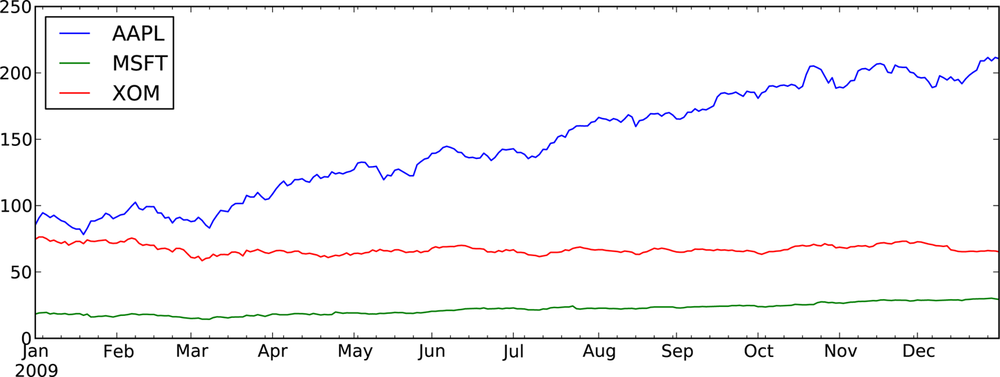
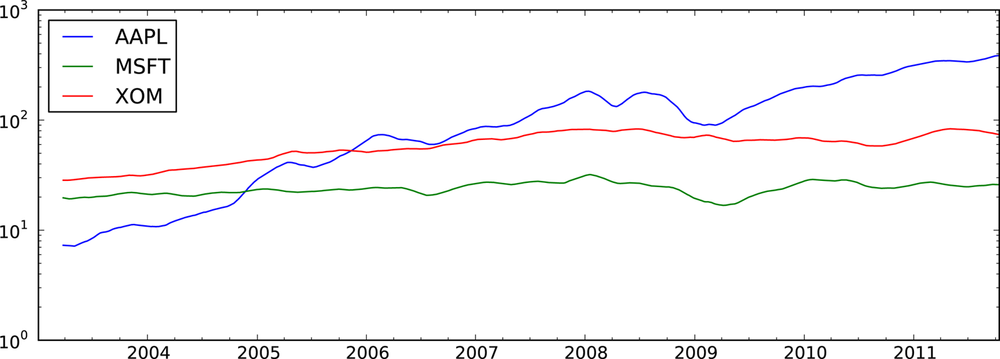
2002Q3 0.046303 0.163344 0.251503 -0.157276Plots with pandas time series have improved date formatting compared with matplotlib out of the box. As an example, I downloaded some stock price data on a few common US stock from Yahoo! Finance:
In [232]: close_px_all = pd.read_csv('ch09/stock_px.csv', parse_dates=True, index_col=0)

In [233]: close_px = close_px_all[['AAPL', 'MSFT', 'XOM']]

In [234]: close_px = close_px.resample('B', fill_method='ffill')

In [235]: close_px.info()
<class 'pandas.core.frame.DataFrame'>
DatetimeIndex: 2292 entries, 2003-01-02 00:00:00 to 2011-10-14 00:00:00
Freq: B
Data columns (total 3 columns):
AAPL    2292 non-null float64
MSFT    2292 non-null float64
XOM     2292 non-null float64
dtypes: float64(3)
Calling plot on one of the
columns grenerates a simple plot, seen in Figure 10-4.
In [237]: close_px['AAPL'].plot()

When called on a DataFrame, as you would expect, all of the time series are drawn on a single subplot with a legend indicating which is which. I’ll plot only the year 2009 data so you can see how both months and years are formatted on the X axis; see Figure 10-5.
In [239]: close_px.ix['2009'].plot()
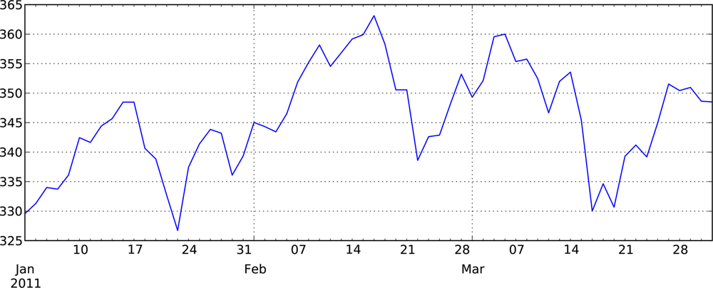
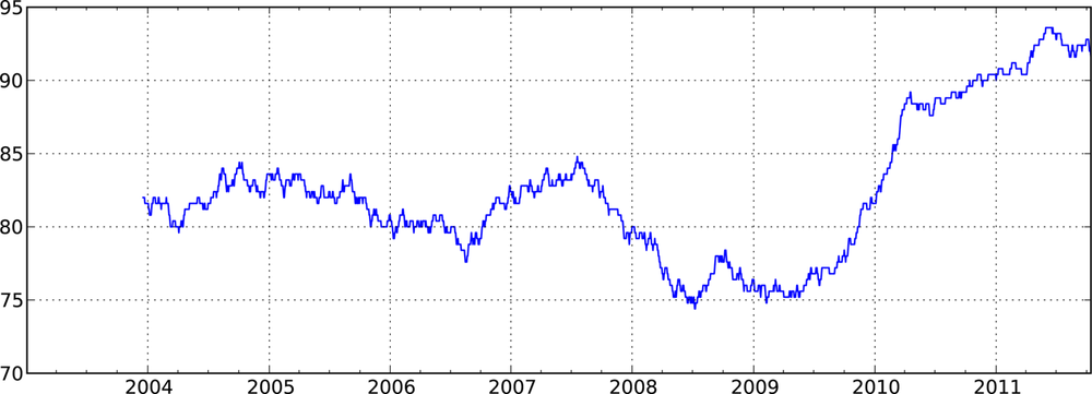
In [241]: close_px['AAPL'].ix['01-2011':'03-2011'].plot()
Quarterly frequency data is also more nicely formatted with quarterly markers, something that would be quite a bit more work to do by hand. See Figure 10-7.
In [243]: appl_q = close_px['AAPL'].resample('Q-DEC', fill_method='ffill')

In [244]: appl_q.ix['2009':].plot()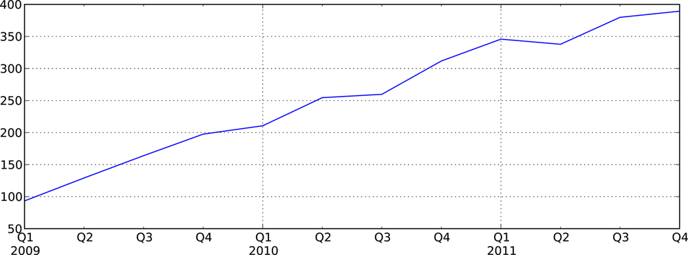
A last feature of time series plotting in pandas is that by right-clicking and dragging to zoom in and out, the dates will be dynamically expanded or contracted and reformatting depending on the timespan contained in the plot view. This is of course only true when using matplotlib in interactive mode.
A common class of array transformations intended for time series operations are statistics and other functions evaluated over a sliding window or with exponentially decaying weights. I call these moving window functions, even though it includes functions without a fixed-length window like exponentially-weighted moving average. Like other statistical functions, these also automatically exclude missing data.
rolling_mean is one of
the simplest such functions. It takes a TimeSeries or DataFrame along with
a window (expressed as a number of
periods):
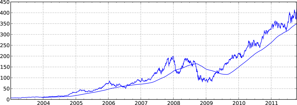
In [248]: close_px.AAPL.plot()
Out[248]: <matplotlib.axes.AxesSubplot at 0xb392ff0c>

In [249]: pd.rolling_mean(close_px.AAPL, 250).plot()
See Figure 10-8 for the plot. By default
functions like rolling_mean require the
indicated number of non-NA observations. This behavior can be changed to
account for missing data and, in particular, the fact that you will have
fewer than window periods of data at
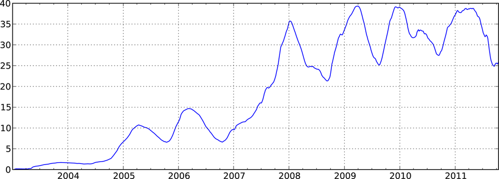
the beginning of the time series (see Figure 10-9):
In [251]: appl_std250 = pd.rolling_std(close_px.AAPL, 250, min_periods=10)

In [252]: appl_std250[5:12]
Out[252]:
2003-01-09         NaN
2003-01-10         NaN
2003-01-13         NaN
2003-01-14         NaN
2003-01-15    0.077496
2003-01-16    0.074760
2003-01-17    0.112368
Freq: B, dtype: float64

In [253]: appl_std250.plot()
To compute an expanding window mean, you can see that an expanding window is just a special case where the window is the length of the time series, but only one or more periods is required to compute a value:
# Define expanding mean in terms of rolling_mean
In [254]: expanding_mean = lambda x: rolling_mean(x, len(x), min_periods=1)
Calling rolling_mean and friends
on a DataFrame applies the transformation to each column (see Figure 10-10):
In [256]: pd.rolling_mean(close_px, 60).plot(logy=True)
See Table 10-6 for a listing of related functions in pandas.
Table 10-6. Moving window and exponentially-weighted functions
Note
bottleneck, a Python
library by Keith Goodman, provides an alternate implementation of
NaN-friendly moving window functions
and may be worth looking at depending on your application.
An alternative to using a static window size with
equally-weighted observations is to specify a constant decay
factor to give more weight to more recent observations. In
mathematical terms, if mat is the moving average result at time t and x is the time series in question, each value in the
result is computed as mat = a * mat -
1 + (1 - a) * xt, where a is the decay factor. There are a couple of ways to
specify the decay factor, a popular one is using a span, which makes the result
comparable to a simple moving window function with window size equal to
the span.
Since an exponentially-weighted statistic places more weight on
more recent observations, it “adapts” faster to changes compared with
the equal-weighted version. Here’s an example comparing a 60-day moving
average of Apple’s stock price with an EW moving average with span=60 (see Figure 10-11):
fig, axes = plt.subplots(nrows=2, ncols=1, sharex=True, sharey=True,
                         figsize=(12, 7))

aapl_px = close_px.AAPL['2005':'2009']

ma60 = pd.rolling_mean(aapl_px, 60, min_periods=50)
ewma60 = pd.ewma(aapl_px, span=60)

aapl_px.plot(style='k-', ax=axes[0])
ma60.plot(style='k--', ax=axes[0])
aapl_px.plot(style='k-', ax=axes[1])
ewma60.plot(style='k--', ax=axes[1])
axes[0].set_title('Simple MA')
axes[1].set_title('Exponentially-weighted MA')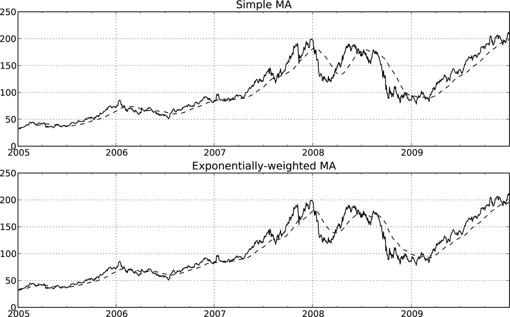
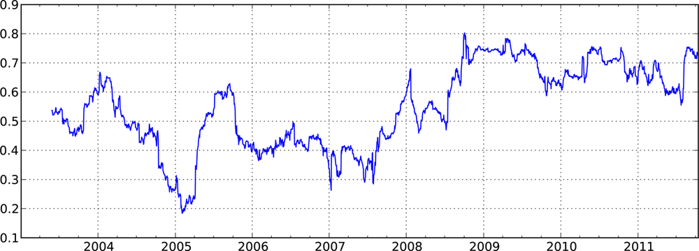
Some statistical operators, like correlation and
covariance, need to operate on two time series. As an example, financial
analysts are often interested in a stock’s correlation to a benchmark
index like the S&P 500. We can compute that by computing the percent
changes and using rolling_corr (see
Figure 10-12):
In [263]: spx_rets = spx_px / spx_px.shift(1) - 1

In [264]: returns = close_px.pct_change()

In [265]: corr = pd.rolling_corr(returns.AAPL, spx_rets, 125, min_periods=100)

In [266]: corr.plot()
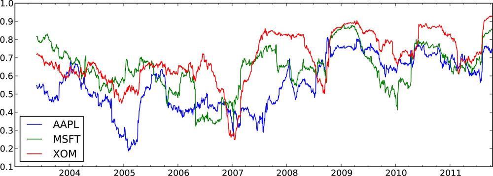
Suppose you wanted to compute the correlation of the S&P 500
index with many stocks at once. Writing a loop and creating a new
DataFrame would be easy but maybe get repetitive, so if you pass a
TimeSeries and a DataFrame, a function like rolling_corr will compute the correlation of
the TimeSeries (spx_rets in this
case) with each column in the DataFrame. See Figure 10-13 for the plot of the result:
In [268]: corr = pd.rolling_corr(returns, spx_rets, 125, min_periods=100)

In [269]: corr.plot()
The rolling_apply function
provides a means to apply an array function of your own devising over a
moving window. The only requirement is that the function produce a
single value (a reduction) from each piece of the array. For example,
while we can compute sample quantiles using rolling_quantile, we
might be interested in the percentile rank of a particular value over
the sample. The scipy.stats.percentileofscore function does
just this:
In [271]: from scipy.stats import percentileofscore

In [272]: score_at_2percent = lambda x: percentileofscore(x, 0.02)

In [273]: result = pd.rolling_apply(returns.AAPL, 250, score_at_2percent)

In [274]: result.plot()
Timestamps and periods are represented as 64-bit integers
using NumPy’s datetime64 dtype. This
means that for each data point, there is an associated 8 bytes of memory
per timestamp. Thus, a time series with 1 million float64 data points has a memory footprint of
approximately 16 megabytes. Since pandas makes every effort to share
indexes among time series, creating views on existing time series do not
cause any more memory to be used. Additionally, indexes for lower
frequencies (daily and up) are stored in a central cache, so that any
fixed-frequency index is a view on the date cache. Thus, if you have a
large collection of low-frequency time series, the memory footprint of the
indexes will not be as significant.
Performance-wise, pandas has been highly optimized for data
alignment operations (the behind-the-scenes work of differently indexed
ts1 + ts2) and resampling. Here is an
example of aggregating 10MM data points to OHLC:
In [275]: rng = pd.date_range('1/1/2000', periods=10000000, freq='10ms')

In [276]: ts = Series(np.random.randn(len(rng)), index=rng)

In [277]: ts
Out[277]:
2000-01-01 00:00:00           1.543222
2000-01-01 00:00:00.010000    0.887621
2000-01-01 00:00:00.020000   -2.043524
2000-01-01 00:00:00.030000   -0.809157
...
2000-01-02 03:46:39.960000   -1.489348
2000-01-02 03:46:39.970000   -0.194531
2000-01-02 03:46:39.980000    0.967617
2000-01-02 03:46:39.990000    1.605598
Freq: 10, Length: 10000000

In [278]: ts.resample('15min', how='ohlc').info()
<class 'pandas.core.frame.DataFrame'>
DatetimeIndex: 112 entries, 2000-01-01 00:00:00 to 2000-01-02 03:45:00
Freq: 15T
Data columns (total 4 columns):
open     112 non-null float64
high     112 non-null float64
low      112 non-null float64
close    112 non-null float64
dtypes: float64(4)
In [279]: %timeit ts.resample('15min', how='ohlc')
10 loops, best of 3: 102 ms per loop
The runtime may depend slightly on the relative size of the aggregated result; higher frequency aggregates unsurprisingly take longer to compute:
In [280]: rng = pd.date_range('1/1/2000', periods=10000000, freq='1s')

In [281]: ts = Series(np.random.randn(len(rng)), index=rng)

In [282]: %timeit ts.resample('15s', how='ohlc')
1 loops, best of 3: 171 ms per loop
It’s possible that by the time you read this, the performance of these algorithms may be even further improved. As an example, there are currently no optimizations for conversions between regular frequencies, but that would be fairly straightforward to do.
[5] The choice of the default values for closed and label might
seem a bit odd to some users. In practice the choice is somewhat
arbitrary; for some target frequencies, closed='left' is preferable, while for
others closed='right' makes more
sense. The important thing is that you keep in mind exactly how you
are segmenting the data.