
Act without doing; work without effort. Think of the small as large and the few as many. Confront the difficult while it is still easy; accomplish the great task by a series of small acts.
—Laozi
People often ask me, “What is your Python development environment?” My answer is almost always the same, “IPython and a text editor”. You may choose to substitute an Integrated Development Environment (IDE) for a text editor in order to take advantage of more advanced graphical tools and code completion capabilities. Even if so, I strongly recommend making IPython an important part of your workflow. Some IDEs even provide IPython integration, so it’s possible to get the best of both worlds.
The IPython project began in 2001 as Fernando Pérez’s side project to make a better interactive Python interpreter. In the subsequent 11 years it has grown into what’s widely considered one of the most important tools in the modern scientific Python computing stack. While it does not provide any computational or data analytical tools by itself, IPython is designed from the ground up to maximize your productivity in both interactive computing and software development. It encourages an execute-explore workflow instead of the typical edit-compile-run workflow of many other programming languages. It also provides very tight integration with the operating system’s shell and file system. Since much of data analysis coding involves exploration, trial and error, and iteration, IPython will, in almost all cases, help you get the job done faster.
Of course, the IPython project now encompasses a great deal more than just an enhanced, interactive Python shell. It also includes a rich GUI console with inline plotting, a web-based interactive notebook format, and a lightweight, fast parallel computing engine. And, as with so many other tools designed for and by programmers, it is highly customizable. I’ll discuss some of these features later in the chapter.
Since IPython has interactivity at its core, some of the features in this chapter are difficult to fully illustrate without a live console. If this is your first time learning about IPython, I recommend that you follow along with the examples to get a feel for how things work. As with any keyboard-driven console-like environment, developing muscle-memory for the common commands is part of the learning curve.
Note
Many parts of this chapter (for example: profiling and debugging) can be safely omitted on a first reading as they are not necessary for understanding the rest of the book. This chapter is intended to provide a standalone, rich overview of the functionality provided by IPython.
You can launch IPython on the command line just like launching the
regular Python interpreter except with the ipython command:
$ ipython
Python 2.7.2 (default, May 27 2012, 21:26:12)
Type "copyright", "credits" or "license" for more information.

IPython 0.12 -- An enhanced Interactive Python.
?         -> Introduction and overview of IPython's features.
%quickref -> Quick reference.
help      -> Python's own help system.
object?   -> Details about 'object', use 'object??' for extra details.

In [1]: a = 5

In [2]: a
Out[2]: 5
You can execute arbitrary Python statements by typing them in and
pressing <return>. When typing
just a variable into IPython, it renders a string representation of the
object:
In [541]: import numpy as np

In [542]: data = {i : np.random.randn() for i in range(7)}

In [543]: data
Out[543]:
{0: 0.6900018528091594,
 1: 1.0015434424937888,
 2: -0.5030873913603446,
 3: -0.6222742250596455,
 4: -0.9211686080130108,
 5: -0.726213492660829,
 6: 0.2228955458351768}
Many kinds of Python objects are formatted
to be more readable, or pretty-printed, which is distinct from
normal printing with print. If you
printed a dict like the above in the standard Python interpreter, it would
be much less readable:
>>> from numpy.random import randn
>>> data = {i : randn() for i in range(7)}
>>> print data
{0: -1.5948255432744511, 1: 0.10569006472787983, 2: 1.972367135977295,
3: 0.15455217573074576, 4: -0.24058577449429575, 5: -1.2904897053651216,
6: 0.3308507317325902}
IPython also provides facilities to make it easy to execute arbitrary blocks of code (via somewhat glorified copy-and-pasting) and whole Python scripts. These will be discussed shortly.
On the surface, the IPython shell looks like a
cosmetically slightly-different interactive Python interpreter. Users of
Mathematica may find the enumerated input and output prompts familiar.
One of the major improvements over the standard Python shell is
tab completion, a feature common to most
interactive data analysis environments. While entering expressions in
the shell, pressing <Tab> will
search the namespace for any variables (objects, functions, etc.)
matching the characters you have typed so far:
In [1]: an_apple = 27

In [2]: an_example = 42

In [3]: an<Tab>
an_apple    and         an_example  any
In this example, note that IPython displayed both the two
variables I defined as well as the Python keyword and and built-in function any. Naturally, you can also complete methods
and attributes on any object after typing a period:
In [3]: b = [1, 2, 3]

In [4]: b.<Tab>
b.append   b.extend   b.insert   b.remove   b.sort
b.count    b.index    b.pop      b.reverse
The same goes for modules:
In [1]: import datetime

In [2]: datetime.<Tab>
datetime.date           datetime.MAXYEAR        datetime.timedelta
datetime.datetime       datetime.MINYEAR        datetime.tzinfo
datetime.datetime_CAPI  datetime.time
Note
Note that IPython by default hides methods and attributes starting with underscores, such as magic methods and internal “private” methods and attributes, in order to avoid cluttering the display (and confusing new Python users!). These, too, can be tab-completed but you must first type an underscore to see them. If you prefer to always see such methods in tab completion, you can change this setting in the IPython configuration.
Tab completion works in many contexts outside of searching the
interactive namespace and completing object or module attributes.When
typing anything that looks like a file path (even in a Python string),
pressing <Tab> will complete
anything on your computer’s file system matching what you’ve
typed:
In [3]: book_scripts/<Tab>book_scripts/cprof_example.py book_scripts/ipython_script_test.py book_scripts/ipython_bug.py book_scripts/prof_mod.py In [3]: path = 'book_scripts/<Tab>book_scripts/cprof_example.py book_scripts/ipython_script_test.py book_scripts/ipython_bug.py book_scripts/prof_mod.py
Combined with the %run command
(see later section), this functionality will undoubtedly save you many
keystrokes.
Another area where tab completion saves time is in the completion
of function keyword arguments (including the = sign!).
Using a question mark (?) before or after a variable will display
some general information about the object:
In [545]: b?
Type:       list
String Form:[1, 2, 3]
Length:     3
Docstring:
list() -> new empty list
list(iterable) -> new list initialized from iterable's items
This is referred to as object introspection. If the object is a function or instance method, the docstring, if defined, will also be shown. Suppose we’d written the following function:
def add_numbers(a, b):
    """
    Add two numbers together

    Returns
    -------
    the_sum : type of arguments
    """
    return a + b
Then using ? shows us the
docstring:
In [547]: add_numbers?
Type:       function
String Form:<function add_numbers at 0x5fad848>
File:       book_scripts/<ipython-input-546-5473012eeb65>
Definition: add_numbers(a, b)
Docstring:
Add two numbers together
Returns
-------
the_sum : type of arguments
Using ?? will also show the
function’s source code if possible:
In [548]: add_numbers??
Type:       function
String Form:<function add_numbers at 0x5fad848>
File:       book_scripts/<ipython-input-546-5473012eeb65>
Definition: add_numbers(a, b)
Source:
def add_numbers(a, b):
    """
    Add two numbers together
    Returns
    -------
    the_sum : type of arguments
    """
    return a + b
? has a final usage,
which is for searching the IPython namespace in a manner similar to the
standard UNIX or Windows command line. A number of characters combined
with the wildcard (*) will show all
names matching the wildcard expression. For example, we could get a list
of all functions in the top level NumPy namespace containing load:
In [549]: np.*load*?
np.load
np.loads
np.loadtxt
np.pkgload
Any file can be run as a Python program inside the
environment of your IPython session using the %run command. Suppose you had the following
simple script stored in ipython_script_test.py:
def f(x, y, z):
    return (x + y) / z

a = 5
b = 6
c = 7.5

result = f(a, b, c)
This can be executed by passing the file name to %run:
In [550]: %run ipython_script_test.py
The script is run in an empty
namespace (with no imports or other variables defined) so
that the behavior should be identical to running the program on the
command line using python script.py.
All of the variables (imports, functions, and globals) defined in the
file (up until an exception, if any, is raised) will then be accessible
in the IPython shell:
In [551]: c
Out[551]: 7.5

In [552]: result
Out[552]: 1.4666666666666666
If a Python script expects command line arguments (to be found in
sys.argv), these can be passed after
the file path as though run on the command line.
Note
Should you wish to give a script access to variables already
defined in the interactive IPython namespace, use %run -i instead of plain %run.
Pressing <Ctrl-C> while any code is running,
whether a script through %run or a
long-running command, will cause a KeyboardInterrupt to
be raised. This will cause nearly all Python programs to stop
immediately except in very exceptional cases.
Warning
When a piece of Python code has called into some compiled
extension modules, pressing <Ctrl-C> will not cause the program
execution to stop immediately in all cases. In such cases, you will
have to either wait until control is returned to the Python
interpreter, or, in more dire circumstances, forcibly terminate the
Python process via the OS task manager.
A quick-and-dirty way to execute code in IPython is via
pasting from the clipboard. This might seem fairly crude, but in
practice it is very useful. For example, while developing a complex or
time-consuming application, you may wish to execute a script piece by
piece, pausing at each stage to examine the currently loaded data and
results. Or, you might find a code snippet on the Internet that you want
to run and play around with, but you’d rather not create a new
.py file for it.
Code snippets can be pasted from the clipboard in many cases by
pressing <Ctrl-Shift-V>. Note
that it is not completely robust as this mode of pasting mimics typing
each line into IPython, and line breaks are treated as <return>. This means that if you paste
code with an indented block and there is a blank line, IPython will
think that the indented block is over. Once the next line in the block
is executed, an IndentationError will
be raised. For example the following code:
x = 5
y = 7
if x > 5:
    x += 1

    y = 8
will not work if simply pasted:
In [1]: x = 5

In [2]: y = 7

In [3]: if x > 5:
   ...:         x += 1
   ...:

In [4]:     y = 8
IndentationError: unexpected indent

If you want to paste code into IPython, try the %paste and %cpaste
magic functions.
As the error message suggests, we should instead use the
%paste and %cpaste magic
functions. %paste takes whatever
text is in the clipboard and executes it as a single block in the
shell:
In [6]: %paste
x = 5
y = 7
if x > 5:
    x += 1

    y = 8
## -- End pasted text --
Caution
Depending on your platform and how you installed Python, there’s
a small chance that %paste will not work.
Packaged distributions like EPDFree (as described in in the intro)
should not be a problem.
%cpaste is similar, except that
it gives you a special prompt for pasting code into:
In [7]: %cpaste
Pasting code; enter '--' alone on the line to stop or use Ctrl-D.
:x = 5
:y = 7
:if x > 5:
:    x += 1
:
:    y = 8
:--
With the %cpaste block, you
have the freedom to paste as much code as you like before executing it.
You might decide to use %cpaste in
order to look at the pasted code before executing it. If you
accidentally paste the wrong code, you can break out of the %cpaste prompt by pressing <Ctrl-C>.
Later, I’ll introduce the IPython HTML Notebook which brings a new level of sophistication for developing analyses block-by-block in a browser-based notebook format with executable code cells.
Some text editors, such as Emacs and vim, have 3rd party extensions enabling blocks of code to be sent directly from the editor to a running IPython shell. Refer to the IPython website or do an Internet search to find out more.
Some IDEs, such as the PyDev plugin for Eclipse and Python Tools for Visual Studio from Microsoft (and possibly others), have integration with the IPython terminal application. If you want to work in an IDE but don’t want to give up the IPython console features, this may be a good option for you.
IPython has many keyboard shortcuts for navigating the prompt (which will be familiar to users of the Emacs text editor or the UNIX bash shell) and interacting with the shell’s command history (see later section). Table 3-1 summarizes some of the most commonly used shortcuts. See Figure 3-1 for an illustration of a few of these, such as cursor movement.
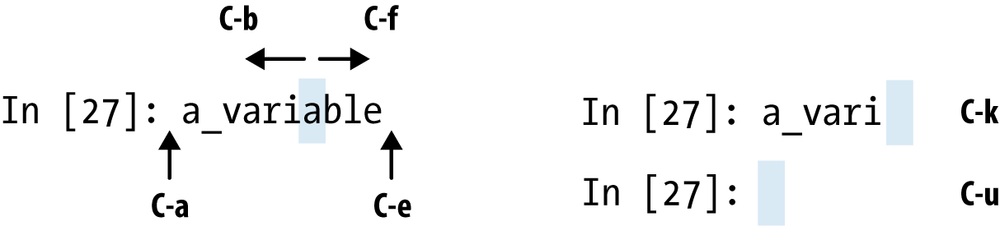
Table 3-1. Standard IPython Keyboard Shortcuts
If an exception is raised while %run-ing a script or executing any statement,
IPython will by default print a full call stack trace (traceback) with a
few lines of context around the position at each point in the
stack.
In [553]: %run ch03/ipython_bug.py
---------------------------------------------------------------------------
AssertionError                            Traceback (most recent call last)
/home/wesm/code/ipython/IPython/utils/py3compat.pyc in execfile(fname, *where)
    176             else:
    177                 filename = fname
--> 178             __builtin__.execfile(filename, *where)
book_scripts/ch03/ipython_bug.py in <module>()
     13     throws_an_exception()
     14
---> 15 calling_things()
book_scripts/ch03/ipython_bug.py in calling_things()
     11 def calling_things():
     12     works_fine()
---> 13     throws_an_exception()
     14
     15 calling_things()
book_scripts/ch03/ipython_bug.py in throws_an_exception()
      7     a = 5
      8     b = 6
----> 9     assert(a + b == 10)
     10
     11 def calling_things():
AssertionError:
Having additional context by itself is a big advantage over the
standard Python interpreter (which does not provide any additional
context). The amount of context shown can be controlled using the
%xmode magic command,
from minimal (same as the standard Python interpreter) to verbose (which
inlines function argument values and more). As you will see later in the
chapter, you can step into the stack (using the
%debug or %pdb magics) after an
error has occurred for interactive post-mortem debugging.
IPython has many special commands, known as “magic”
commands, which are designed to facilitate common tasks and enable you
to easily control the behavior of the IPython system. A magic command is
any command prefixed by the the percent symbol %. For example, you can check the execution
time of any Python statement, such as a matrix multiplication, using the
%timeit magic function
(which will be discussed in more detail later):
In [554]: a = np.random.randn(100, 100)

In [555]: %timeit np.dot(a, a)
10000 loops, best of 3: 69.1 us per loop
Magic commands can be viewed as command line programs to be run
within the IPython system. Many of them have additional “command line”
options, which can all be viewed (as you might expect) using ?:
In [1]: %reset?
Resets the namespace by removing all names defined by the user.

Parameters
----------
  -f : force reset without asking for confirmation.

  -s : 'Soft' reset: Only clears your namespace, leaving history intact.
  References to objects may be kept. By default (without this option),
  we do a 'hard' reset, giving you a new session and removing all
  references to objects from the current session.

Examples
--------
In [6]: a = 1

In [7]: a
Out[7]: 1

In [8]: %reset -f

In [10]: a
---------------------------------------------------------------------------
NameError                                 Traceback (most recent call last)
<ipython-input-10-60b725f10c9c> in <module>()
----> 1 a

NameError: name 'a' is not defined
Magic functions can be used by default without the percent sign,
as long as no variable is defined with the same name as the magic
function in question. This feature is called
automagic and can be enabled or disabled using
%automagic.
Since IPython’s documentation is easily accessible from within the
system, I encourage you to explore all of the special commands available
by typing %quickref or %magic. I will
highlight a few more of the most critical ones for being productive in
interactive computing and Python development in IPython.
Table 3-2. Frequently-used IPython Magic Commands
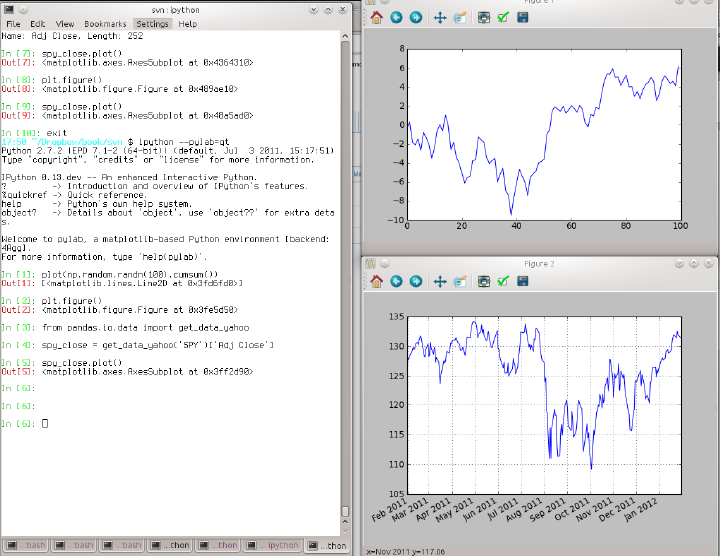
The IPython team has developed a Qt framework-based GUI console, designed to wed the features of the terminal-only applications with the features provided by a rich text widget, like embedded images, multiline editing, and syntax highlighting. If you have either PyQt or PySide installed, the application can be launched with inline plotting by running this on the command line:
ipython qtconsole --pylab=inline
The Qt console can launch multiple IPython processes in tabs, enabling you to switch between tasks. It can also share a process with the IPython HTML Notebook application, which I’ll highlight later.
Part of why IPython is so widely used in scientific computing is that it is designed as a companion to libraries like matplotlib and other GUI toolkits. Don’t worry if you have never used matplotlib before; it will be discussed in much more detail later in this book. If you create a matplotlib plot window in the regular Python shell, you’ll be sad to find that the GUI event loop “takes control” of the Python session until the plot window is closed. That won’t work for interactive data analysis and visualization, so IPython has implemented special handling for each GUI framework so that it will work seamlessly with the shell.
The typical way to launch IPython with matplotlib integration is
by adding the --pylab flag (two
dashes).
$ ipython --pylab
This will cause several things to happen. First IPython will
launch with the default GUI backend integration enabled so that
matplotlib plot windows can be created with no issues. Secondly, most of
NumPy and matplotlib will be imported into the top level interactive
namespace to produce an interactive computing environment reminiscent of
MATLAB and other domain-specific scientific computing environments. It’s
possible to do this setup by hand by using %gui, too (try running
%gui? to find out how).
IPython maintains a small on-disk database containing the text of each command that you execute. This serves various purposes:
Searching, completing, and executing previously-executed commands with minimal typing
Persisting the command history between sessions.
Logging the input/output history to a file
Being able to search and execute previous commands is, for
many people, the most useful feature. Since IPython encourages an
iterative, interactive code development workflow, you may often find
yourself repeating the same commands, such as a %run command or some other code snippet.
Suppose you had run:
In[7]: %run first/second/third/data_script.py
and then explored the results of the script (assuming it ran
successfully), only to find that you made an incorrect calculation.
After figuring out the problem and modifying data_script.py, you can start typing a few
letters of the %run command then
press either the <Ctrl-P> key
combination or the <up arrow>
key. This will search the command history for the first prior command
matching the letters you typed. Pressing either <Ctrl-P> or <up arrow> multiple times will continue
to search through the history. If you pass over the command you wish to
execute, fear not. You can move forward through the
command history by pressing either <Ctrl-N> or <down arrow>. After doing this a few
times you may start pressing these keys without thinking!
Using <Ctrl-R> gives you
the same partial incremental searching capability provided by the
readline used in UNIX-style shells,
such as the bash shell. On Windows, readline functionality
is emulated by IPython. To use this, press <Ctrl-R> then type a few characters
contained in the input line you want to search for:
In [1]: a_command = foo(x, y, z)

(reverse-i-search)`com': a_command = foo(x, y, z)
Pressing <Ctrl-R> will
cycle through the history for each line matching the characters you’ve
typed.
Forgetting to assign the result of a function call to a
variable can be very annoying. Fortunately, IPython stores references to
both the input (the text that you type) and output
(the object that is returned) in special variables. The previous two
outputs are stored in the _ (one underscore) and
__ (two underscores)
variables, respectively:
In [556]: 2 ** 27
Out[556]: 134217728

In [557]: _
Out[557]: 134217728
Input variables are stored in variables named like _iX, where X is the input line number. For each such
input variables there is a corresponding output variable _X. So after input line 27, say, there will be
two new variables _27 (for the
output) and _i27 for the
input.
In [26]: foo = 'bar'

In [27]: foo
Out[27]: 'bar'

In [28]: _i27
Out[28]: u'foo'

In [29]: _27
Out[29]: 'bar'
Since the input variables are strings, that can be executed again
using the Python exec keyword:
In [30]: exec _i27
Several magic functions allow you to work with the input and
output history. %hist is capable of
printing all or part of the input history, with or without line numbers.
%reset is for clearing
the interactive namespace and optionally the input and output caches.
The %xdel magic function is
intended for removing all references to a
particular object from the IPython machinery. See
the documentation for both of these magics for more details.
Warning
When working with very large data sets, keep in mind that
IPython’s input and output history causes any object referenced there
to not be garbage collected (freeing up the memory), even if you
delete the variables from the interactive namespace using the
del keyword. In such
cases, careful usage of %xdel and %reset can help you
avoid running into memory problems.
IPython is capable of logging the entire console session
including input and output. Logging is turned on by typing %logstart:
In [3]: %logstart
Activating auto-logging. Current session state plus future input saved.
Filename       : ipython_log.py
Mode           : rotate
Output logging : False
Raw input log  : False
Timestamping   : False
State          : active
IPython logging can be enabled at any time and it will record your
entire session (including previous commands). Thus, if you are working
on something and you decide you want to save everything you did, you can
simply enable logging. See the docstring of %logstart for more
options (including changing the output file path), as well as the
companion functions %logoff, %logon,
%logstate, and %logstop.
Another important feature of IPython is that it provides very strong integration with the operating system shell. This means, among other things, that you can perform most standard command line actions as you would in the Windows or UNIX (Linux, OS X) shell without having to exit IPython. This includes executing shell commands, changing directories, and storing the results of a command in a Python object (list or string). There are also simple shell command aliasing and directory bookmarking features.
See Table 3-3 for a summary of magic functions and syntax for calling shell commands. I’ll briefly visit these features in the next few sections.
Table 3-3. IPython system-related commands
Starting a line in IPython with an exclamation point
!, or bang, tells
IPython to execute everything after the bang in the system shell. This
means that you can delete files (using rm or del,
depending on your OS), change directories, or execute any other process.
It’s even possible to start processes that take control away from
IPython, even another Python interpreter:
In [2]: !python
Python 2.7.2 |EPD 7.1-2 (64-bit)| (default, Jul  3 2011, 15:17:51)
[GCC 4.1.2 20080704 (Red Hat 4.1.2-44)] on linux2
Type "packages", "demo" or "enthought" for more information.
>>>
The console output of a shell command can be stored in a variable
by assigning the !-escaped expression to
a variable. For example, on my Linux-based machine connected to the
Internet via ethernet, I can get my IP address as a Python
variable:
In [1]: ip_info = !ifconfig eth0 | grep "inet "

In [2]: ip_info[0].strip()
Out[2]: 'inet addr:192.168.1.137  Bcast:192.168.1.255  Mask:255.255.255.0'
The returned Python object ip_info is actually a custom list type
containing various versions of the console output.
IPython can also substitute in Python values defined in the
current environment when using !. To
do this, preface the variable name by the dollar sign $:
In [3]: foo = 'test*'

In [4]: !ls $foo
test4.py  test.py  test.xml
The %alias magic function
can define custom shortcuts for shell commands. As a simple
example:
In [1]: %alias ll ls -l

In [2]: ll /usr
total 332
drwxr-xr-x   2 root root  69632 2012-01-29 20:36 bin/
drwxr-xr-x   2 root root   4096 2010-08-23 12:05 games/
drwxr-xr-x 123 root root  20480 2011-12-26 18:08 include/
drwxr-xr-x 265 root root 126976 2012-01-29 20:36 lib/
drwxr-xr-x  44 root root  69632 2011-12-26 18:08 lib32/
lrwxrwxrwx   1 root root      3 2010-08-23 16:02 lib64 -> lib/
drwxr-xr-x  15 root root   4096 2011-10-13 19:03 local/
drwxr-xr-x   2 root root  12288 2012-01-12 09:32 sbin/
drwxr-xr-x 387 root root  12288 2011-11-04 22:53 share/
drwxrwsr-x  24 root src    4096 2011-07-17 18:38 src/
Multiple commands can be executed just as on the command line by separating them with semicolons:
In [558]: %alias test_alias (cd ch08; ls; cd ..)

In [559]: test_alias
macrodata.csv  spx.csv	tips.csv
You’ll notice that IPython “forgets” any aliases you define interactively as soon as the session is closed. To create permanent aliases, you will need to use the configuration system. See later in the chapter.
IPython has a simple directory bookmarking system to enable you to save aliases for common directories so that you can jump around very easily. For example, I’m an avid user of Dropbox, so I can define a bookmark to make it easy to change directories to my Dropbox:
In [6]: %bookmark db /home/wesm/Dropbox/
Once I’ve done this, when I use the %cd magic, I can use any bookmarks I’ve
defined
In [7]: cd db
(bookmark:db) -> /home/wesm/Dropbox/
/home/wesm/Dropbox
If a bookmark name conflicts with a directory name in your current
working directory, you can use the -b
flag to override and use the bookmark location. Using the -l option with %bookmark lists all of
your bookmarks:
In [8]: %bookmark -l
Current bookmarks:
db -> /home/wesm/Dropbox/
Bookmarks, unlike aliases, are automatically persisted between IPython sessions.
In addition to being a comfortable environment for
interactive computing and data exploration, IPython is well suited as a
software development environment. In data analysis applications, it’s
important first to have correct code. Fortunately,
IPython has closely integrated and enhanced the built-in Python pdb debugger. Secondly
you want your code to be fast. For this IPython has
easy-to-use code timing and profiling tools. I will give an overview of
these tools in detail here.
IPython’s debugger enhances pdb with tab
completion, syntax highlighting, and context for each line in exception
tracebacks. One of the best times to debug code is right after an error
has occurred. The %debug command, when
entered immediately after an exception, invokes the “post-mortem”
debugger and drops you into the stack frame where the exception was
raised:
In [2]: run ch03/ipython_bug.py
---------------------------------------------------------------------------
AssertionError                            Traceback (most recent call last)
/home/wesm/book_scripts/ch03/ipython_bug.py in <module>()
     13     throws_an_exception()
     14
---> 15 calling_things()

/home/wesm/book_scripts/ch03/ipython_bug.py in calling_things()
     11 def calling_things():
     12     works_fine()
---> 13     throws_an_exception()
     14
     15 calling_things()

/home/wesm/book_scripts/ch03/ipython_bug.py in throws_an_exception()
      7     a = 5
      8     b = 6
----> 9     assert(a + b == 10)
     10
     11 def calling_things():

AssertionError:

In [3]: %debug
> /home/wesm/book_scripts/ch03/ipython_bug.py(9)throws_an_exception()
      8     b = 6
----> 9     assert(a + b == 10)
     10

ipdb>
Once inside the debugger, you can execute arbitrary Python code
and explore all of the objects and data (which have been “kept alive” by
the interpreter) inside each stack frame. By default you start in the
lowest level, where the error occurred. By pressing u (up) and d (down), you can switch between the levels of
the stack trace:
ipdb> u
> /home/wesm/book_scripts/ch03/ipython_bug.py(13)calling_things()
     12     works_fine()
---> 13     throws_an_exception()
     14
Executing the %pdb command makes it
so that IPython automatically invokes the debugger after any exception,
a mode that many users will find especially useful.
It’s also easy to use the debugger to help develop code,
especially when you wish to set breakpoints or step through the
execution of a function or script to examine the state at each stage.
There are several ways to accomplish this. The first is by using
%run with the -d flag, which invokes the debugger before
executing any code in the passed script. You must immediately press
s (step) to enter the script:
In [5]: run -d ch03/ipython_bug.py
Breakpoint 1 at /home/wesm/book_scripts/ch03/ipython_bug.py:1
NOTE: Enter 'c' at the ipdb>  prompt to start your script.
> <string>(1)<module>()

ipdb> s
--Call--
> /home/wesm/book_scripts/ch03/ipython_bug.py(1)<module>()
1---> 1 def works_fine():
      2     a = 5
      3     b = 6
After this point, it’s up to you how you want to work your way
through the file. For example, in the above exception, we could set a
breakpoint right before calling the works_fine method and run the script until we
reach the breakpoint by pressing c
(continue):
ipdb> b 12
ipdb> c
> /home/wesm/book_scripts/ch03/ipython_bug.py(12)calling_things()
     11 def calling_things():
2--> 12     works_fine()
     13     throws_an_exception()
At this point, you can step
into works_fine() or execute works_fine() by pressing n (next) to advance to the next line:
ipdb> n
> /home/wesm/book_scripts/ch03/ipython_bug.py(13)calling_things()
2    12     works_fine()
---> 13     throws_an_exception()
     14
Then, we could step into throws_an_exception and advance to the line
where the error occurs and look at the variables in the scope. Note that
debugger commands take precedence over variable names; in such cases
preface the variables with ! to examine their
contents.
ipdb> s
--Call--
> /home/wesm/book_scripts/ch03/ipython_bug.py(6)throws_an_exception()
      5
----> 6 def throws_an_exception():
      7     a = 5

ipdb> n
> /home/wesm/book_scripts/ch03/ipython_bug.py(7)throws_an_exception()
      6 def throws_an_exception():
----> 7     a = 5
      8     b = 6

ipdb> n
> /home/wesm/book_scripts/ch03/ipython_bug.py(8)throws_an_exception()
      7     a = 5
----> 8     b = 6
      9     assert(a + b == 10)

ipdb> n
> /home/wesm/book_scripts/ch03/ipython_bug.py(9)throws_an_exception()
      8     b = 6
----> 9     assert(a + b == 10)
     10

ipdb> !a
5
ipdb> !b
6
Becoming proficient in the interactive debugger is largely a matter of practice and experience. See Table 3-4 for a full catalogue of the debugger commands. If you are used to an IDE, you might find the terminal-driven debugger to be a bit bewildering at first, but that will improve in time. Most of the Python IDEs have excellent GUI debuggers, but it is usually a significant productivity gain to remain in IPython for your debugging.
Table 3-4. (I)Python debugger commands
There are a couple of other useful ways to invoke the debugger.
The first is by using a special set_trace function
(named after pdb.set_trace), which
is basically a “poor man’s breakpoint”. Here are two small recipes you
might want to put somewhere for your general use (potentially adding
them to your IPython profile as I do):
def set_trace():
    from IPython.core.debugger import Pdb
    Pdb(color_scheme='Linux').set_trace(sys._getframe().f_back)

def debug(f, *args, **kwargs):
    from IPython.core.debugger import Pdb
    pdb = Pdb(color_scheme='Linux')
    return pdb.runcall(f, *args, **kwargs)
The first function, set_trace, is very
simple. Put set_trace() anywhere
in your code that you want to stop and take a look around (for
example, right before an exception occurs):
In [7]: run ch03/ipython_bug.py
> /home/wesm/book_scripts/ch03/ipython_bug.py(16)calling_things()
     15     set_trace()
---> 16     throws_an_exception()
     17
Pressing c (continue) will
cause the code to resume normally with no harm done.
The debug function above
enables you to invoke the interactive debugger easily on an arbitrary
function call. Suppose we had written a function like
def f(x, y, z=1):
    tmp = x + y
    return tmp / z
and we wished to step through its logic. Ordinarily using
f would look like f(1, 2, z=3). To instead step into f, pass f
as the first argument to debug followed by the
positional and keyword arguments to be passed to f:
In [6]: debug(f, 1, 2, z=3)
> <ipython-input>(2)f()
      1 def f(x, y, z):
----> 2     tmp = x + y
      3     return tmp / z

ipdb>
I find that these two simple recipes save me a lot of time on a day-to-day basis.
Lastly, the debugger can be used in conjunction with %run. By running a script with %run -d, you will be dropped directly into
the debugger, ready to set any breakpoints and start the
script:
In [1]: %run -d ch03/ipython_bug.py
Breakpoint 1 at /home/wesm/book_scripts/ch03/ipython_bug.py:1
NOTE: Enter 'c' at the ipdb>  prompt to start your script.
> <string>(1)<module>()

ipdb>
Adding -b with a line number
starts the debugger with a breakpoint set already:
In [2]: %run -d -b2 ch03/ipython_bug.py
Breakpoint 1 at /home/wesm/book_scripts/ch03/ipython_bug.py:2
NOTE: Enter 'c' at the ipdb>  prompt to start your script.
> <string>(1)<module>()

ipdb> c
> /home/wesm/book_scripts/ch03/ipython_bug.py(2)works_fine()
      1 def works_fine():
1---> 2     a = 5
      3     b = 6

ipdb>For larger-scale or longer-running data analysis applications, you may wish to measure the execution time of various components or of individual statements or function calls. You may want a report of which functions are taking up the most time in a complex process. Fortunately, IPython enables you to get this information very easily while you are developing and testing your code.
Timing code by hand using the built-in time module and its functions time.clock and time.time is often tedious and repetitive, as
you must write the same uninteresting boilerplate code:
import time
start = time.time()
for i in range(iterations):
    # some code to run here
elapsed_per = (time.time() - start) / iterations
Since this is such a common operation, IPython has two magic
functions %time and %timeit to automate
this process for you. %time runs a statement
once, reporting the total execution time. Suppose we had a large list of
strings and we wanted to compare different methods of selecting all
strings starting with a particular prefix. Here is a simple list of
600,000 strings and two identical methods of selecting only the ones
that start with 'foo':
# a very large list of strings
strings = ['foo', 'foobar', 'baz', 'qux',
           'python', 'Guido Van Rossum'] * 100000

method1 = [x for x in strings if x.startswith('foo')]

method2 = [x for x in strings if x[:3] == 'foo']
It looks like they should be about the same performance-wise,
right? We can check for sure using %time:
In [561]: %time method1 = [x for x in strings if x.startswith('foo')]
CPU times: user 0.19 s, sys: 0.00 s, total: 0.19 s
Wall time: 0.19 s

In [562]: %time method2 = [x for x in strings if x[:3] == 'foo']
CPU times: user 0.09 s, sys: 0.00 s, total: 0.09 s
Wall time: 0.09 s
The Wall time is the main
number of interest. So, it looks like the first method takes more than
twice as long, but it’s not a very precise measurement. If you try
%time-ing those
statements multiple times yourself, you’ll find that the results are
somewhat variable. To get a more precise measurement, use the %timeit magic function.
Given an arbitrary statement, it has a heuristic to run a statement
multiple times to produce a fairly accurate average runtime.
In [563]: %timeit [x for x in strings if x.startswith('foo')]
10 loops, best of 3: 159 ms per loop

In [564]: %timeit [x for x in strings if x[:3] == 'foo']
10 loops, best of 3: 59.3 ms per loop
This seemingly innocuous example illustrates that it is worth understanding the performance characteristics of the Python standard library, NumPy, pandas, and other libraries used in this book. In larger-scale data analysis applications, those milliseconds will start to add up!
%timeit is especially
useful for analyzing statements and functions with very short execution
times, even at the level of microseconds (1e-6 seconds) or nanoseconds
(1e-9 seconds). These may seem like insignificant amounts of time, but
of course a 20 microsecond function invoked 1 million times takes 15
seconds longer than a 5 microsecond function. In the above example, we
could very directly compare the two string operations to understand
their performance characteristics:
In [565]: x = 'foobar'

In [566]: y = 'foo'

In [567]: %timeit x.startswith(y)
1000000 loops, best of 3: 267 ns per loop

In [568]: %timeit x[:3] == y
10000000 loops, best of 3: 147 ns per loop
Profiling code is closely related to timing code, except
it is concerned with determining where time is
spent. The main Python profiling tool is the cProfile module, which is not specific to
IPython at all. cProfile executes a
program or any arbitrary block of code while keeping track of how much
time is spent in each function.
A common way to use cProfile is
on the command line, running an entire program and outputting the
aggregated time per function. Suppose we had a simple script which does
some linear algebra in a loop (computing the maximum absolute
eigenvalues of a series of 100 x 100
matrices):
import numpy as np
from numpy.linalg import eigvals

def run_experiment(niter=100):
    K = 100
    results = []
    for _ in xrange(niter):
        mat = np.random.randn(K, K)
        max_eigenvalue = np.abs(eigvals(mat)).max()
        results.append(max_eigenvalue)
    return results
some_results = run_experiment()
print 'Largest one we saw: %s' % np.max(some_results)
Don’t worry if you are not familiar with NumPy. You can run this
script through cProfile by running
the following in the command line:
python -m cProfile cprof_example.py
If you try that, you’ll find that the results are outputted sorted
by function name. This makes it a bit hard to get an idea of where the
most time is spent, so it’s very common to specify a sort
order using the -s
flag:
$ python -m cProfile -s cumulative cprof_example.py
Largest one we saw: 11.923204422
    15116 function calls (14927 primitive calls) in 0.720 seconds

Ordered by: cumulative time

ncalls  tottime  percall  cumtime  percall filename:lineno(function)
     1    0.001    0.001    0.721    0.721 cprof_example.py:1(<module>)
   100    0.003    0.000    0.586    0.006 linalg.py:702(eigvals)
   200    0.572    0.003    0.572    0.003 {numpy.linalg.lapack_lite.dgeev}
     1    0.002    0.002    0.075    0.075 __init__.py:106(<module>)
   100    0.059    0.001    0.059    0.001 {method 'randn')
     1    0.000    0.000    0.044    0.044 add_newdocs.py:9(<module>)
     2    0.001    0.001    0.037    0.019 __init__.py:1(<module>)
     2    0.003    0.002    0.030    0.015 __init__.py:2(<module>)
     1    0.000    0.000    0.030    0.030 type_check.py:3(<module>)
     1    0.001    0.001    0.021    0.021 __init__.py:15(<module>)
     1    0.013    0.013    0.013    0.013 numeric.py:1(<module>)
     1    0.000    0.000    0.009    0.009 __init__.py:6(<module>)
     1    0.001    0.001    0.008    0.008 __init__.py:45(<module>)
   262    0.005    0.000    0.007    0.000 function_base.py:3178(add_newdoc)
   100    0.003    0.000    0.005    0.000 linalg.py:162(_assertFinite)
   ...
Only the first 15 rows of the output are shown. It’s easiest to
read by scanning down the cumtime
column to see how much total time was spent inside
each function. Note that if a function calls some other function,
the clock does not stop running. cProfile records the start and end time of
each function call and uses that to produce the timing.
In addition to the above command-line usage, cProfile can also be used programmatically to
profile arbitrary blocks of code without having to run a new process.
IPython has a convenient interface to this capability using the %prun command and the -p option to %run. %prun
takes the same “command line options” as cProfile but will profile an arbitrary Python
statement instead of a whole .py
file:
In [4]: %prun -l 7 -s cumulative run_experiment()
         4203 function calls in 0.643 seconds

Ordered by: cumulative time
List reduced from 32 to 7 due to restriction <7>

ncalls  tottime  percall  cumtime  percall filename:lineno(function)
     1    0.000    0.000    0.643    0.643 <string>:1(<module>)
     1    0.001    0.001    0.643    0.643 cprof_example.py:4(run_experiment)
   100    0.003    0.000    0.583    0.006 linalg.py:702(eigvals)
   200    0.569    0.003    0.569    0.003 {numpy.linalg.lapack_lite.dgeev}
   100    0.058    0.001    0.058    0.001 {method 'randn'}
   100    0.003    0.000    0.005    0.000 linalg.py:162(_assertFinite)
   200    0.002    0.000    0.002    0.000 {method 'all' of 'numpy.ndarray' objects}
Similarly, calling %run -p -s cumulative
cprof_example.py has the same effect as the command-line
approach above, except you never have to leave IPython.
In some cases the information you obtain from %prun (or another cProfile-based profile method) may not tell
the whole story about a function’s execution time, or it may be so
complex that the results, aggregated by function name, are hard to
interpret. For this case, there is a small library called line_profiler (obtainable via PyPI or one of
the package management tools). It contains an IPython extension enabling
a new magic function %lprun that computes a
line-by-line-profiling of one or more functions. You can enable this
extension by modifying your IPython configuration (see the IPython
documentation or the section on configuration later in this chapter) to
include the following line:
# A list of dotted module names of IPython extensions to load.
c.TerminalIPythonApp.extensions = ['line_profiler']
line_profiler can be
used programmatically (see the full documentation), but it is perhaps
most powerful when used interactively in IPython. Suppose you had a
module prof_mod with the following
code doing some NumPy array operations:
from numpy.random import randn

def add_and_sum(x, y):
    added = x + y
    summed = added.sum(axis=1)
    return summed

def call_function():
    x = randn(1000, 1000)
    y = randn(1000, 1000)
    return add_and_sum(x, y)
If we wanted to understand the performance of the add_and_sum function, %prun gives us the
following:
In [569]: %run prof_mod

In [570]: x = randn(3000, 3000)

In [571]: y = randn(3000, 3000)

In [572]: %prun add_and_sum(x, y)
         4 function calls in 0.049 seconds
   Ordered by: internal time
   ncalls  tottime  percall  cumtime  percall filename:lineno(function)
        1    0.036    0.036    0.046    0.046 prof_mod.py:3(add_and_sum)
        1    0.009    0.009    0.009    0.009 {method 'sum' of 'numpy.ndarray' objects}
        1    0.003    0.003    0.049    0.049 <string>:1(<module>)
        1    0.000    0.000    0.000    0.000 {method 'disable' of '_lsprof.Profiler' objects}
This is not especially enlightening. With the line_profiler IPython extension activated, a
new command %lprun is available. The
only difference in usage is that we must instruct %lprun which function or functions we wish to
profile. The general syntax is:
%lprun -f func1 -f func2 statement_to_profileIn this case, we want to profile add_and_sum, so we run:
In [573]: %lprun -f add_and_sum add_and_sum(x, y)
Timer unit: 1e-06 s
File: book_scripts/prof_mod.py
Function: add_and_sum at line 3
Total time: 0.045936 s
Line #      Hits         Time  Per Hit   % Time  Line Contents
==============================================================
     3                                           def add_and_sum(x, y):
     4         1        36510  36510.0     79.5      added = x + y
     5         1         9425   9425.0     20.5      summed = added.sum(axis=1)
     6         1            1      1.0      0.0      return summed
You’ll probably agree this is much easier to interpret. In this
case we profiled the same function we used in the statement. Looking at
the module code above, we could call call_function and profile that as well as
add_and_sum, thus getting a full
picture of the performance of the code:
In [574]: %lprun -f add_and_sum -f call_function call_function()
Timer unit: 1e-06 s
File: book_scripts/prof_mod.py
Function: add_and_sum at line 3
Total time: 0.005526 s
Line #      Hits         Time  Per Hit   % Time  Line Contents
==============================================================
     3                                           def add_and_sum(x, y):
     4         1         4375   4375.0     79.2      added = x + y
     5         1         1149   1149.0     20.8      summed = added.sum(axis=1)
     6         1            2      2.0      0.0      return summed
File: book_scripts/prof_mod.py
Function: call_function at line 8
Total time: 0.121016 s
Line #      Hits         Time  Per Hit   % Time  Line Contents
==============================================================
     8                                           def call_function():
     9         1        57169  57169.0     47.2      x = randn(1000, 1000)
    10         1        58304  58304.0     48.2      y = randn(1000, 1000)
    11         1         5543   5543.0      4.6      return add_and_sum(x, y)
As a general rule of thumb, I tend to prefer %prun (cProfile) for “macro” profiling and %lprun (line_profiler) for “micro” profiling. It’s
worthwhile to have a good understanding of both tools.
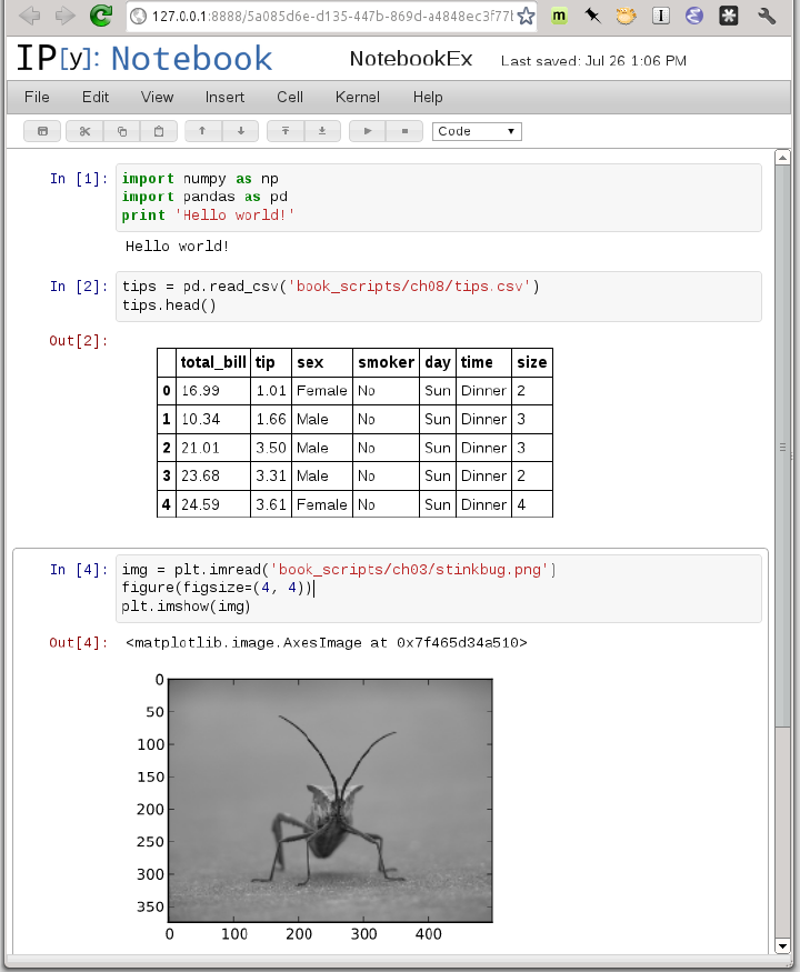
Starting in 2011, the IPython team, led by Brian Granger, built a web technology−based interactive computational document format that is commonly known as the IPython Notebook. It has grown into a wonderful tool for interactive computing and an ideal medium for reproducible research and teaching. I’ve used it while writing most of the examples in the book; I encourage you to make use of it, too.
It has a JSON-based .ipynb document format
that enables easy sharing of code, output, and figures. Recently in Python
conferences, a popular approach for demonstrations has been to use the
notebook and post the .ipynb files online
afterward for everyone to play with.
The notebook application runs as a lightweight server process on the command line. It can be started by running:
$ ipython notebook --pylab=inline
[NotebookApp] Using existing profile dir: u'/home/wesm/.config/ipython/profile_default'
[NotebookApp] Serving notebooks from /home/wesm/book_scripts
[NotebookApp] The IPython Notebook is running at: http://127.0.0.1:8888/
[NotebookApp] Use Control-C to stop this server and shut down all kernels.
On most platforms, your primary web browser will automatically open up to the notebook dashboard. In some cases you may have to navigate to the listed URL. From there, you can create a new notebook and start exploring.
Since you use the notebook inside a web browser, the server process can run anywhere. You can even securely connect to notebooks running on cloud service providers like Amazon EC2. As of this writing, a new project NotebookCloud (http://notebookcloud.appspot.com) makes it easy to launch notebooks on EC2.
Writing code in a way that makes it easy to develop, debug, and ultimately use interactively may be a paradigm shift for many users. There are procedural details like code reloading that may require some adjustment as well as coding style concerns.
As such, most of this section is more of an art than a science and will require some experimentation on your part to determine a way to write your Python code that is effective and productive for you. Ultimately you want to structure your code in a way that makes it easy to use iteratively and to be able to explore the results of running a program or function as effortlessly as possible. I have found software designed with IPython in mind to be easier to work with than code intended only to be run as as standalone command-line application. This becomes especially important when something goes wrong and you have to diagnose an error in code that you or someone else might have written months or years beforehand.
In Python, when you type import
some_lib, the code in some_lib is executed and all the variables,
functions, and imports defined within are stored in the newly created
some_lib module namespace. The next
time you type import some_lib, you
will get a reference to the existing module namespace. The potential
difficulty in interactive code development in IPython comes when you,
say, %run a script that depends on
some other module where you may have made changes. Suppose I had the
following code in test_script.py:
import some_lib x = 5 y = [1, 2, 3, 4] result = some_lib.get_answer(x, y)
If you were to execute %run
test_script.py then modify some_lib.py, the next time you execute
%run test_script.py you will still
get the old version of some_lib because of Python’s “load-once”
module system. This behavior differs from some other data analysis
environments, like MATLAB, which automatically propagate code
changes.[2] To cope with this, you have a couple of options. The first
way is to use Python’s built-in reload function,
altering test_script.py to look like
the following:
import some_lib
reload(some_lib)

x = 5
y = [1, 2, 3, 4]
result = some_lib.get_answer(x, y)
This guarantees that you will get a fresh copy of some_lib every time you run test_script.py. Obviously, if the dependencies
go deeper, it might be a bit tricky to be inserting usages of reload all over the
place. For this problem, IPython has a special dreload function
(not a magic function) for “deep” (recursive)
reloading of modules. If I were to run import
some_lib then type dreload(some_lib), it will attempt to reload
some_lib as well as all of its
dependencies. This will not work in all cases, unfortunately, but when
it does it beats having to restart IPython.
There’s no simple recipe for this, but here are some high-level principles I have found effective in my own work.
It’s not unusual to see a program written for the command line with a structure somewhat like the following trivial example:
from my_functions import g

def f(x, y):
    return g(x + y)

def main():
    x = 6
    y = 7.5
    result = x + y

if __name__ == '__main__':
    main()
Do you see what might be wrong with this program if we were to
run it in IPython? After it’s done, none of the results or objects
defined in the main function will be
accessible in the IPython shell. A better way is to have whatever code
is in main execute directly
in the module’s global namespace (or in the if __name__ == '__main__': block, if you
want the module to also be importable). That way, when you %run the code, you’ll be able to look at all
of the variables defined in main.
It’s less meaningful in this simple example, but in this book we’ll be
looking at some complex data analysis problems involving large data
sets that you will want to be able to play with in IPython.
Deeply nested code makes me think about the many layers of an onion. When testing or debugging a function, how many layers of the onion must you peel back in order to reach the code of interest? The idea that “flat is better than nested” is a part of the Zen of Python, and it applies generally to developing code for interactive use as well. Making functions and classes as decoupled and modular as possible makes them easier to test (if you are writing unit tests), debug, and use interactively.
If you come from a Java (or another such language) background, you may have been told to keep files short. In many languages, this is sound advice; long length is usually a bad “code smell”, indicating refactoring or reorganization may be necessary. However, while developing code using IPython, working with 10 small, but interconnected files (under, say, 100 lines each) is likely to cause you more headache in general than a single large file or two or three longer files. Fewer files means fewer modules to reload and less jumping between files while editing, too. I have found maintaining larger modules, each with high internal cohesion, to be much more useful and pythonic. After iterating toward a solution, it sometimes will make sense to refactor larger files into smaller ones.
Obviously, I don’t support taking this argument to the extreme, which would to be to put all of your code in a single monstrous file. Finding a sensible and intuitive module and package structure for a large codebase often takes a bit of work, but it is especially important to get right in teams. Each module should be internally cohesive, and it should be as obvious as possible where to find functions and classes responsible for each area of functionality.
IPython makes every effort to display a console-friendly
string representation of any object that you inspect. For many objects,
like dicts, lists, and tuples, the built-in pprint module is used
to do the nice formatting. In user-defined classes, however, you have to
generate the desired string output yourself. Suppose we had the
following simple class:
class Message:
    def __init__(self, msg):
        self.msg = msg
If you wrote this, you would be disappointed to discover that the default output for your class isn’t very nice:
In [576]: x = Message('I have a secret')

In [577]: x
Out[577]: <__main__.Message instance at 0x60ebbd8>
IPython takes the string returned by the __repr__ magic method (by doing output = repr(obj)) and prints that to the
console. Thus, we can add a simple __repr__ method to the above class to get a
more helpful output:
class Message:
    def __init__(self, msg):
        self.msg = msg

    def __repr__(self):
        return 'Message: %s' % self.msg
In [579]: x = Message('I have a secret')
In [580]: x
Out[580]: Message: I have a secretMost aspects of the appearance (colors, prompt, spacing between lines, etc.) and behavior of the IPython shell are configurable through an extensive configuration system. Here are some of the things you can do via configuration:
Change the color scheme
Change how the input and output prompts look, or remove the blank line after
Outand before the nextInpromptExecute an arbitrary list of Python statements. These could be imports that you use all the time or anything else you want to happen each time you launch IPython
Enable IPython extensions, like the
%lprunmagic inline_profilerDefine your own magics or system aliases
All of these configuration options are specified in a special
ipython_config.py file
which will be found in the ~/.config/ipython/ directory on UNIX-like
systems and %HOME%/.ipython/
directory on Windows. Where your home directory is depends on your
system. Configuration is performed based on a particular profile. When you start IPython
normally, you load up, by default, the default
profile, stored in the profile_default
directory. Thus, on my Linux OS the full path to my default IPython
configuration file is:
/home/wesm/.config/ipython/profile_default/ipython_config.py
I’ll spare you the gory details of what’s in this file. Fortunately it has comments describing what each configuration option is for, so I will leave it to the reader to tinker and customize. One additional useful feature is that it’s possible to have multiple profiles. Suppose you wanted to have an alternate IPython configuration tailored for a particular application or project. Creating a new profile is as simple is typing something like
ipython profile create secret_project
Once you’ve done this, edit the config files in the newly-created
profile_secret_project directory then
launch IPython like so
$ ipython --profile=secret_project
Python 2.7.2 |EPD 7.1-2 (64-bit)| (default, Jul  3 2011, 15:17:51)
Type "copyright", "credits" or "license" for more information.

IPython 0.13 -- An enhanced Interactive Python.
?         -> Introduction and overview of IPython's features.
%quickref -> Quick reference.
help      -> Python's own help system.
object?   -> Details about 'object', use 'object??' for extra details.

IPython profile: secret_project

In [1]:
As always, the online IPython documentation is an excellent resource for more on profiles and configuration.
Parts of this chapter were derived from the wonderful documentation put together by the IPython Development Team. I can’t thank them enough for all of their work building this amazing set of tools.
[2] Since a module or package may be imported in many different places in a particular program, Python caches a module’s code the first time it is imported rather than executing the code in the module every time. Otherwise, modularity and good code organization could potentially cause inefficiency in an application.