
Appendix C. Py Sci
In her reign the power of steam
On land and sea became supreme,
And all now have strong reliance
In fresh victories of science.James McIntyre, Queen’s Jubilee Ode 1887
In the past few years, largely because of the software you’ll see in this appendix, Python has become extremely popular with scientists. If you’re a scientist or student yourself, you might have used tools like MATLAB and R, or traditional languages such as Java, C, or C++. In this appendix, you’ll see how Python makes an excellent platform for scientific analysis and publishing.
Math and Statistics in the Standard Library
First, let’s take a little trip back to the standard library and visit some features and modules that we’ve ignored.
Math Functions
Python has a menagerie of math functions in the standard
math library.
Just type import math to access them from your programs.
It has a few constants such as pi and e:
>>>importmath>>>math.pi>>>3.141592653589793>>>math.e2.718281828459045
Most of it consists of functions, so let’s look at the most useful ones.
fabs() returns the absolute value of its argument:
>>>math.fabs(98.6)98.6>>>math.fabs(-271.1)271.1
Get the integer below (floor()) and above (ceil()) some number:
>>>math.floor(98.6)98>>>math.floor(-271.1)-272>>>math.ceil(98.6)99>>>math.ceil(-271.1)-271
Calculate the factorial (in math, n !) by using factorial():
>>>math.factorial(0)1>>>math.factorial(1)1>>>math.factorial(2)2>>>math.factorial(3)6>>>math.factorial(10)3628800
Get the logarithm of the argument in base e with log():
>>>math.log(1.0)0.0>>>math.log(math.e)1.0
If you want a different base for the log, provide it as a second argument:
>>>math.log(8,2)3.0
The function pow() does the opposite,
raising a number to a power:
>>>math.pow(2,3)8.0
Python also has the built-in exponentiation operator ** to do the same,
but it doesn’t automatically convert the result to a float
if the base and power are both integers:
>>>2**38>>>2.0**38.0
Get a square root with sqrt():
>>>math.sqrt(100.0)10.0
Don’t try to trick this function; it’s seen it all before:
>>>math.sqrt(-100.0)Traceback (most recent call last):File"<stdin>", line1, in<module>ValueError:math domain error
The usual trigonometric functions are all there,
and I’ll just list their names here:
sin(), cos(), tan(), asin(), acos(), atan(), and atan2().
If you remember the Pythagorean theorem
(or can say it fast three times without spitting),
the math library also has a hypot() function to calculate the
hypotenuse from two sides:
>>>x=3.0>>>y=4.0>>>math.hypot(x,y)5.0
If you don’t trust all these fancy functions, you can work it out yourself:
>>>math.sqrt(x*x+y*y)5.0>>>math.sqrt(x**2+y**2)5.0
A last set of functions converts angular coordinates:
>>>math.radians(180.0)3.141592653589793>>>math.degrees(math.pi)180.0
Working with Complex Numbers
Complex numbers are fully supported in the base Python language, with their familiar notation of real and imaginary parts:
>>># a real number...55>>># an imaginary number...8j8j>>># an imaginary number...3+2j(3+2j)
Because the imaginary number i (1j in Python) is defined as the
square root of –1, we can execute the following:
>>>1j*1j(-1+0j)>>>(7+1j)*1j(-1+7j)
Some complex math functions are in the standard
cmath
module.
Calculate Accurate Floating Point with decimal
Floating-point numbers in computers are not quite like the real numbers we learned in school. Because computer CPUs are designed for binary math, numbers that aren’t exact powers of two often can’t be represented exactly:
>>>x=10.0/3.0>>>x3.3333333333333335
Whoa, what’s that 5 at the end?
It should be 3 all the way down.
With Python’s
decimal module,
you can represent numbers to your desired level of significance.
This is especially important for calculations involving money.
US currency doesn’t go lower than a cent (a hundredth of a dollar),
so if we’re calculating money amounts as dollars and cents,
we want to be accurate to the penny.
If we try to represent dollars and cents through floating-point values
such as 19.99 and 0.06,
we’ll lose some significance way down in the end bits
before we even begin calculating with them. How do we handle this? Easy. We use the decimal
module, instead:
>>>fromdecimalimportDecimal>>>price=Decimal('19.99')>>>tax=Decimal('0.06')>>>total=price+(price*tax)>>>totalDecimal('21.1894')
We created the price and tax with string values to preserve their significance.
The total calculation maintained all the significant fractions of a cent,
but we want to get the nearest cent:
>>>penny=Decimal('0.01')>>>total.quantize(penny)Decimal('21.19')
You might get the same results with plain old floats and rounding, but not always. You could also multiply everything by 100 and use integer cents in your calculations, but that will bite you eventually, too. There’s a nice discussion of these issues at www.itmaybeahack.com.
Perform Rational Arithmetic with fractions
You can represent numbers as a numerator divided by a denominator
through the standard Python
fractions
module. Here is a simple operation multiplying one-third by
two-thirds:
>>>fromfractionsimportFraction>>>Fraction(1,3)*Fraction(2,3)Fraction(2, 9)
Floating-point arguments can be inexact, so you can use Decimal
within Fraction:
>>>Fraction(1.0/3.0)Fraction(6004799503160661, 18014398509481984)>>>Fraction(Decimal('1.0')/Decimal('3.0'))Fraction(3333333333333333333333333333, 10000000000000000000000000000)
Get the greatest common divisor of two numbers with the gcd function:
>>>importfractions>>>fractions.gcd(24,16)8
Use Packed Sequences with array
A Python list is more like a linked list than an array.
If you want a one-dimensional sequence of the same type,
use the array type.
It uses less space than a list
and supports many list methods.
Create one with
array( typecode , initializer ).
The typecode specifies the data type (like int or float)
and the optional initializer contains initial values, which you can
specify as a list, string, or iterable.
I’ve never used this package for real work. It’s a low-level data structure, useful for things such as image data. If you actually need an array—especially with more then one dimension—to do numeric calculations, you’re much better off with NumPy, which we’ll discuss momentarily.
Handling Simple Stats by Using statistics
Beginning with Python 3.4,
statistics
is a standard module.
It has the usual functions: mean, media, mode, standard deviation, variance, and so on.
Input arguments are sequences (lists or tuples) or iterators
of various numeric data types: int, float, decimal, and fraction.
One function, mode, also accepts strings.
Many more statistical functions are available in packages such as SciPy and Pandas, featured later in this appendix.
Matrix Multiplication
Starting with Python 3.5,
you’ll see the @ character
doing something out of character.
It will still be used for decorators,
but it will also have a new use for
matrix multiplication.
However, until it arrives,
NumPy (coming right up)
is your best bet.
Scientific Python
The rest of this appendix covers third-party Python packages for science and math. Although you can install them individually, you should consider downloading all of them at once as part of a scientific Python distribution. Here are your main choices:
- Anaconda
-
This package is free, extensive, up-to-the-minute, supports Python 2 and 3, and won’t clobber your existing system Python.
- Enthought Canopy
-
This package is available in both free and commercial versions.
- Python(x,y)
-
This is a Windows-only release.
- Pyzo
-
This package is based on some tools from Anaconda, plus a few others.
- ALGORETE Loopy
-
This is also based on Anaconda, with extras.
I recommend installing Anaconda. It’s big, but everything in this appendix is in there. See Appendix D for details on using Python 3 with Anaconda. The examples in the rest of this appendix will assume that you’ve installed the required packages, either individually or as part of Anaconda.
NumPy
NumPy is one of the main reasons for Python’s popularity among scientists. You’ve heard that dynamic languages such as Python are often slower than compiled languages like C, or even other interpreted languages such as Java. NumPy was written to provide fast multidimensional numeric arrays, similar to scientific languages like FORTRAN. You get the speed of C with the developer-friendliness of Python.
If you’ve downloaded one of the scientific distributions, you already have NumPy. If not, follow the instructions on the NumPy download page.
To begin with NumPy, you should understand a core data structure, a multidimensional array called an ndarray
(for N-dimensional array)
or just an array.
Unlike Python’s lists and tuples,
each element needs to be of the same type.
NumPy refers to an array’s number of dimensions as its rank.
A one-dimensional array is like a row of values,
a two-dimensional array is like a table of rows and columns,
and a three-dimensional array is like a Rubik’s Cube.
The lengths of the dimensions need not be the same.
Note
The NumPy array and the standard Python array are not the same thing.
For the rest of this appendix,
when I say array, I’m referring to a NumPy array.
But why do you need an array?
-
Scientific data often consists of large sequences of data.
-
Scientific calculations on this data often use matrix math, regression, simulation, and other techniques that process many data points at a time.
-
NumPy handles arrays much faster than standard Python lists or tuples.
There are many ways to make a NumPy array.
Make an Array with array()
You can make an array from a normal list or tuple:
>>>b=np.array([2,4,6,8])>>>barray([2, 4, 6, 8])
The attribute ndim returns the rank:
>>>b.ndim1
The total number of values in the array are given by size:
>>>b.size4
The number of values in each rank are returned by shape:
>>>b.shape(4,)
Make an Array with arange()
NumPy’s arange() method is similar to Python’s standard range().
If you call arange() with a single integer argument num,
it returns an ndarray from 0 to num-1:
>>>importnumpyasnp>>>a=np.arange(10)>>>aarray([0, 1, 2, 3, 4, 5, 6, 7, 8, 9])>>>a.ndim1>>>a.shape(10,)>>>a.size10
With two values, it creates an array from the first to the last minus one:
>>>a=np.arange(7,11)>>>aarray([ 7, 8, 9, 10])
And you can provide a step size to use instead of one as a third argument:
>>>a=np.arange(7,11,2)>>>aarray([7, 9])
So far, our examples have used integers, but floats work just fine:
>>>f=np.arange(2.0,9.8,0.3)>>>farray([ 2. , 2.3, 2.6, 2.9, 3.2, 3.5, 3.8, 4.1, 4.4, 4.7, 5. ,5.3, 5.6, 5.9, 6.2, 6.5, 6.8, 7.1, 7.4, 7.7, 8. , 8.3,8.6, 8.9, 9.2, 9.5, 9.8])
And one last trick:
the dtype argument tells arange what type of values to produce:
>>>g=np.arange(10,4,-1.5,dtype=np.float)>>>garray([ 10. , 8.5, 7. , 5.5])
Make an Array with zeros(), ones(), or random()
The zeros() method returns an array in which all the values are zero.
The argument you provide is a tuple with the shape that you want.
Here’s a one-dimensional array:
>>>a=np.zeros((3,))>>>aarray([ 0., 0., 0.])>>>a.ndim1>>>a.shape(3,)>>>a.size3
This one is of rank two:
>>>b=np.zeros((2,4))>>>barray([[ 0., 0., 0., 0.],[ 0., 0., 0., 0.]])>>>b.ndim2>>>b.shape(2, 4)>>>b.size8
The other special function that fills an array with the same value is ones():
>>>importnumpyasnp>>>k=np.ones((3,5))>>>karray([[ 1., 1., 1., 1., 1.],[ 1., 1., 1., 1., 1.],[ 1., 1., 1., 1., 1.]])
One last initializer creates an array with random values between 0.0 and 1.0:
>>>m=np.random.random((3,5))>>>marray([[ 1.92415699e-01, 4.43131404e-01, 7.99226773e-01,1.14301942e-01, 2.85383430e-04],[ 6.53705749e-01, 7.48034559e-01, 4.49463241e-01,4.87906915e-01, 9.34341118e-01],[ 9.47575562e-01, 2.21152583e-01, 2.49031209e-01,3.46190961e-01, 8.94842676e-01]])
Change an Array’s Shape with reshape()
So far, an array doesn’t seem that different from a list or tuple.
One difference is that you can get it to do tricks, such as change its shape by using reshape():
>>>a=np.arange(10)>>>aarray([0, 1, 2, 3, 4, 5, 6, 7, 8, 9])>>>a=a.reshape(2,5)>>>aarray([[0, 1, 2, 3, 4],[5, 6, 7, 8, 9]])>>>a.ndim2>>>a.shape(2, 5)>>>a.size10
You can reshape the same array in different ways:
>>>a=a.reshape(5,2)>>>aarray([[0, 1],[2, 3],[4, 5],[6, 7],[8, 9]])>>>a.ndim2>>>a.shape(5, 2)>>>a.size10
Assigning a shapely tuple to shape does the same thing:
>>>a.shape=(2,5)>>>aarray([[0, 1, 2, 3, 4],[5, 6, 7, 8, 9]])
The only restriction on a shape is that the product of the rank sizes needs to equal the total number of values (in this case, 10):
>>>a=a.reshape(3,4)Traceback (most recent call last):File"<stdin>", line1, in<module>ValueError:total size of new array must be unchanged
Get an Element with []
A one-dimensional array works like a list:
>>>a=np.arange(10)>>>a[7]7>>>a[-1]9
However, if the array has a different shape, use comma-separated indices:
>>>a.shape=(2,5)>>>aarray([[0, 1, 2, 3, 4],[5, 6, 7, 8, 9]])>>>a[1,2]7
That’s different from a two-dimensional Python list:
>>>l=[[0,1,2,3,4],[5,6,7,8,9]]>>>l[[0, 1, 2, 3, 4], [5, 6, 7, 8, 9]]>>>l[1,2]Traceback (most recent call last):File"<stdin>", line1, in<module>TypeError:list indices must be integers, not tuple>>>l[1][2]7
One last thing: slices work, but again, only within one set of square brackets. Let’s make our familiar test array again:
>>>a=np.arange(10)>>>a=a.reshape(2,5)>>>aarray([[0,1,2,3,4],[5,6,7,8,9]])
Use a slice to get the first row, elements from offset 2 to the end:
>>>a[0,2:]array([2, 3, 4])
Now, get the last row, elements up to the third from the end:
>>>a[-1,:3]array([5, 6, 7])
You can also assign a value to more than one element with a slice.
The following statement assigns the value 1000 to columns (offsets)
2 and 3 of all rows:
>>>a[:,2:4]=1000>>>aarray([[ 0, 1, 1000, 1000, 4],[ 5, 6, 1000, 1000, 9]])
Array Math
Making and reshaping arrays was so much fun that we almost forgot to
actually do something with them.
For our first trick,
we’ll use NumPy’s redefined multiplication (*) operator
to multiply all the values in a NumPy array at once:
>>>fromnumpyimport*>>>a=arange(4)>>>aarray([0, 1, 2, 3])>>>a*=3>>>aarray([0, 3, 6, 9])
If you tried to multiply each element in a normal Python list by a number, you’d need a loop or a list comprehension:
>>>plain_list=list(range(4))>>>plain_list[0, 1, 2, 3]>>>plain_list=[num*3fornuminplain_list]>>>plain_list[0, 3, 6, 9]
This all-at-once behavior also applies to addition, subtraction, division,
and other functions in the NumPy library.
For example, you can initialize all members of an array to any value
by using zeros() and +:
>>>fromnumpyimport*>>>a=zeros((2,5))+17.0>>>aarray([[ 17., 17., 17., 17., 17.],[ 17., 17., 17., 17., 17.]])
Linear Algebra
NumPy includes many functions for linear algebra. For example, let’s define this system of linear equations:
4x + 5y = 20
 x + 2y = 13
How do we solve for x and y?
We’ll build two arrays:
-
The coefficients (multipliers for
xandy) -
The dependent variables (right side of the equation)
>>>importnumpyasnp>>>coefficients=np.array([[4,5],[1,2]])>>>dependents=np.array([20,13])
Now, use the solve() function in the linalg module:
>>>answers=np.linalg.solve(coefficients,dependents)>>>answersarray([ -8.33333333, 10.66666667])
The result says that x is about –8.3 and y is about 10.6.
Did these numbers solve the equation?
>>>4*answers[0]+5*answers[1]20.0>>>1*answers[0]+2*answers[1]13.0
How about that. To avoid all that typing, you can also ask NumPy to get the dot product of the arrays for you:
>>>product=np.dot(coefficients,answers)>>>productarray([ 20., 13.])
The values in the product array should be close to the values in dependents
if this solution is correct.
You can use the allclose() function to check whether the arrays are approximately equal
(they might not be exactly equal because of floating-point rounding):
>>>np.allclose(product,dependents)True
NumPy also has modules for polynomials, Fourier transforms, statistics, and some probability distributions.
The SciPy Library
There’s even more in a library of mathematical and statistical functions built on top of NumPy: SciPy. The SciPy release includes NumPy, SciPy, Pandas (coming later in this appendix), and other libraries.
SciPy includes many modules, including some for the following tasks:
-
Optimization
-
Statistics
-
Interpolation
-
Linear regression
-
Integration
-
Image processing
-
Signal processing
If you’ve worked with other scientific computing tools, you’ll find that Python, NumPy, and SciPy cover some of the same ground as the commercial MATLAB or open source R.
The SciKit Library
In the same pattern of building on earlier software, SciKit is a group of scientific packages built on SciPy. SciKit’s specialty is machine learning: it supports modeling, classification, clustering, and various algorithms.
The IPython Library
IPython is worth your time for many reasons. Here are some of them:
-
An improved interactive interpreter (an alternative to the
>>>examples that we’ve used throughout this book) -
Publishing code, plots, text, and other media in web-based notebooks
-
Support for parallel computing
Let’s look at the interpreter and notebooks.
A Better Interpreter
IPython has different versions for Python 2 and 3,
and both are installed by Anaconda
or other modern scientific Python releases.
Use ipython3 for the Python 3 version.
$ ipython3
Python 3.3.3 (v3.3.3:c3896275c0f6, Nov 16 2013, 23:39:35)
Type "copyright", "credits" or "license" for more information.

IPython 0.13.1 -- An enhanced Interactive Python.
?         -> Introduction and overview of IPython's features.
%quickref -> Quick reference.
help      -> Python's own help system.
object?   -> Details about 'object', use 'object??' for extra details.

In [1]:
The standard Python interpreter uses the input prompts
>>>
and
... to indicate where and when you should type code.
IPython tracks everything you type in a list called In, and all your
output in Out.
Each input can be more than one line, so you submit it by holding
the Shift key while pressing Enter.
Here’s a one-line example:
In [1]: print("Hello? World?")
Hello? World?

In [2]:
In and Out are automatically numbered lists, letting you access any
of the inputs you typed or outputs you received.
If you type ? after a variable, IPython tells you its type, value,
ways of making a variable of that type, and some explanation:
In [4]: answer = 42

In [5]: answer?
Type:       int
String Form:42
Docstring:
int(x=0) -> integer
int(x, base=10) -> integer

Convert a number or string to an integer, or return 0 if no arguments
are given.  If x is a number, return x.__int__().  For floating point
numbers, this truncates towards zero.

If x is not a number or if base is given, then x must be a string,
bytes, or bytearray instance representing an integer literal in the
given base.  The literal can be preceded by '+' or '-' and be surrounded
by whitespace.  The base defaults to 10.  Valid bases are 0 and 2-36.
Base 0 means to interpret the base from the string as an integer literal.
>>> int('0b100', base=0)
4
Name lookup is a popular feature of IDEs such as IPython.
If you press the Tab key right after some characters,
IPython shows all variables, keywords, and functions that begin with those characters.
Let’s define some variables and then find everything that begins with the letter f:
In [6]: fee = 1

In [7]: fie = 2

In [8]: fo = 3

In [9]: fum = 4

In [10]: ftab
%%file    fie       finally   fo        format    frozenset
fee       filter    float     for       from      fum
If you type fe followed by the Tab key, it expands to the variable fee,
which, in this program, is the only thing that starts with fe:
In [11]: fee
Out[11]: 1
IPython Notebook
If you prefer graphical interfaces, you might enjoy IPython’s web-based implementation. You start from the Anaconda launcher window (Figure C-1).
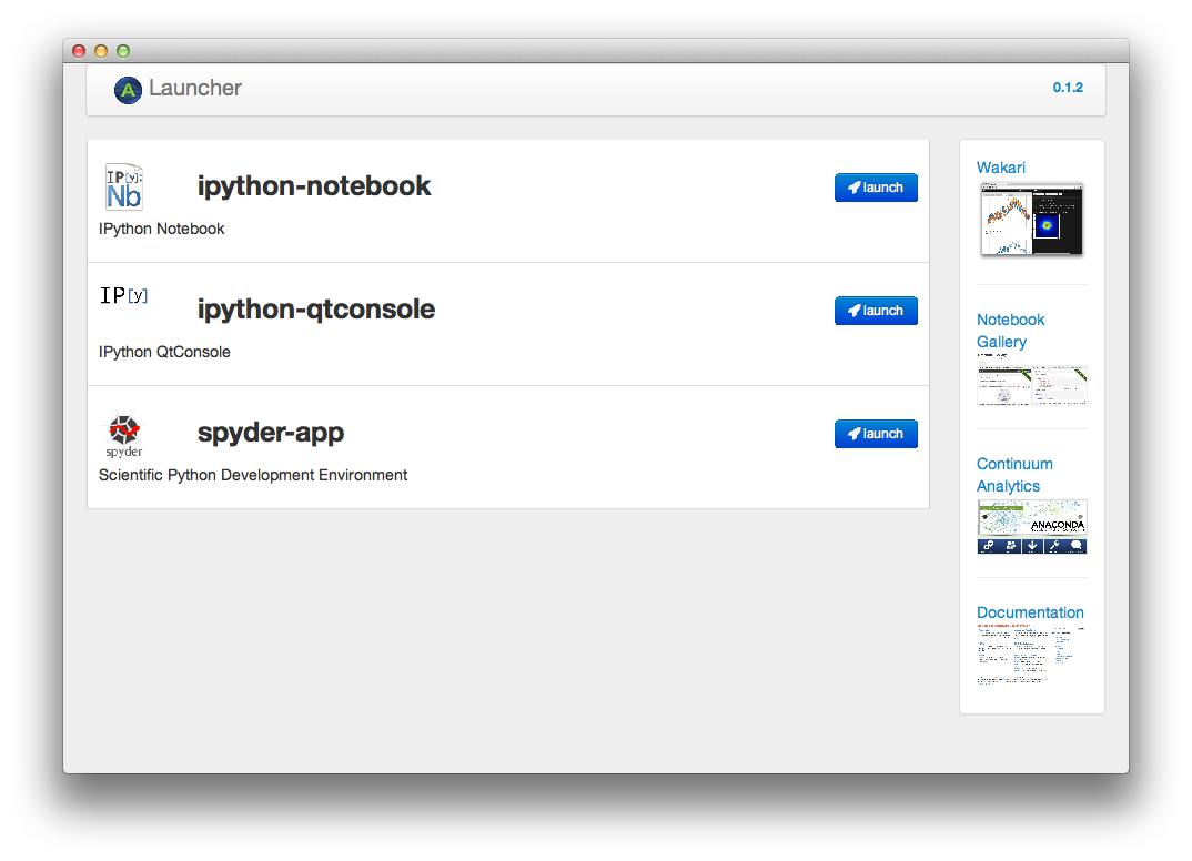
Figure C-1. The Anaconda home page
To launch the notebook in a web browser, click the “launch” icon to the right of “ipython-notebook.” Figure C-2 shows the initial display.
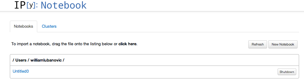
Figure C-2. The iPython home page
Now, click the New Notebook button. A window similar to Figure C-3 opens.
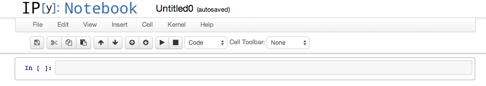
Figure C-3. The iPython Notebook page
For a graphical version of our previous text-based example, type the same command that we used in the previous section, as shown in Figure C-4.
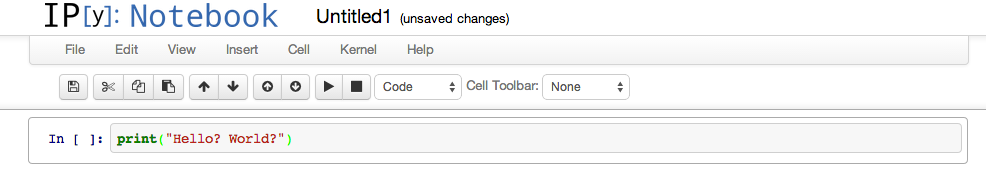
Figure C-4. Entering code in iPython
Click the solid black triangle icon to run it. The result is depicted in Figure C-5.
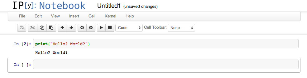
Figure C-5. Running code in iPython
The notebook is more than just a graphical version of an improved interpreter. Besides code, it can contain text, images, and formatted mathematical expressions.
In the row of icons at the top of the notebook, there’s a pull-down menu (Figure C-6) that specifies how you can enter content. Here are the choices:
- Code
-
The default, for Python code
- Markdown
-
An alternative to HTML that serves as readable text and a preprocessor format
- Raw Text
-
Unformatted text Heading 1 through Heading 6: HTML
<H1>through<H6>heading tags
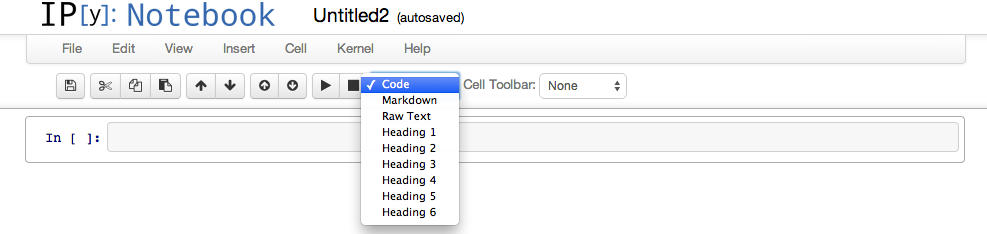
Figure C-6. Menu of content choices
Let’s intersperse some text with our code, making it sort of a wiki. Select Heading 1 from the pull-down menu, type “Humble Brag Example,” and then hold the Shift key while pressing the Enter key. You should see those three words in a large bold font. Then, select Code from the pull-down menu and type some code like this:
print("Some people say this code is ingenious")
Again, press Shift + Enter to complete this entry. You should now see your formatted title and code, as shown in Figure C-7.
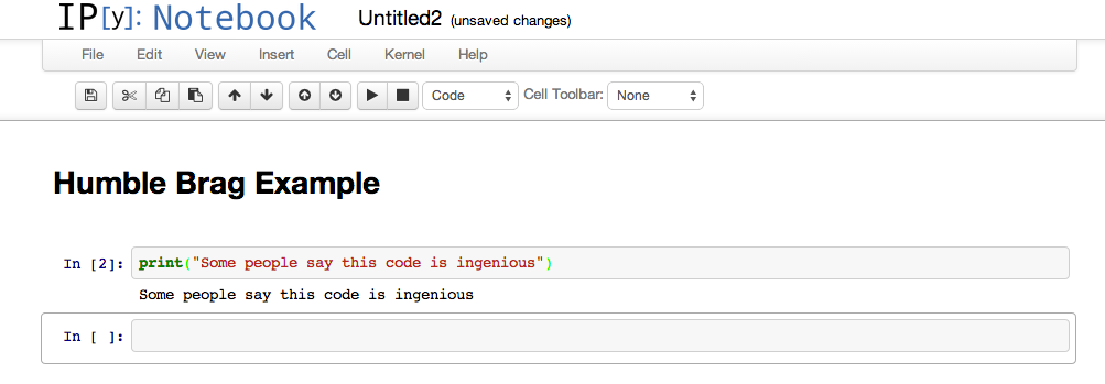
Figure C-7. Formatted text and code
By interspersing code input, output results, text, and even images, you can create an interactive notebook. Because it’s served over the Web, you can access it from any browser.
You can see some notebooks converted to static HTML or in a gallery. For a specific example, try the notebook about the passengers on the Titanic. It includes charts showing how gender, wealth, and position on the ship affected survival. As a bonus, you can read how to apply different machine learning techniques.
Scientists are starting to use IPython notebooks to publish their research, including all the code and data used to reach their conclusions.
Pandas
Recently, the phrase data science has become common. Some definitions that I’ve seen include “statistics done on a Mac,” or “statistics done in San Francisco.” However you define it, the tools we’ve talked about in this chapter—NumPy, SciPy, and the subject of this section, Pandas—are components of a growing popular data-science toolkit. (Mac and San Francisco are optional.)
Pandas is a new package for interactive data analysis. It’s especially useful for real world data manipulation, combining the matrix math of NumPy with the processing ability of spreadsheets and relational databases. The book Python for Data Analysis: Data Wrangling with Pandas, NumPy, and IPython by Wes McKinney (O’Reilly) covers data wrangling with NumPy, IPython, and Pandas.
NumPy is oriented toward traditional scientific computing,
which tends to manipulate multidimensional data sets of a single type,
usually floating point.
Pandas is more like a database editor, handling multiple data types in groups.
In some languages, such groups are called records or structures.
Pandas defines a base data structure called a DataFrame.
This is an ordered collection of columns with names and types.
It has some resemblance to a database table, a Python named tuple,
and a Python nested dictionary.
Its purpose is to simplify the handling of the kind of data you’re
likely to encounter not just in science, but also in business.
In fact, Pandas was originally designed to manipulate financial data,
for which the most common alternative is a spreadsheet.
Pandas is an ETL tool for real world, messy data—missing values, oddball formats, scattered measurements—of all data types. You can split, join, extend, fill in, convert, reshape, slice, and load and save files. It integrates with the tools we’ve just discussed—NumPy, SciPy, iPython—to calculate statistics, fit data to models, draw plots, publish, and so on.
Most scientists just want to get their work done, without spending months to become experts in esoteric computer languages or applications. With Python, they can become productive more quickly.
Python and Scientific Areas
We’ve been looking at Python tools that could be used in almost any area of science. What about software and documentation targeted to specific scientific domains? Here’s a small sample of Python’s use for specific problems, and some special-purpose libraries:
- General
- Physics
- Biology and medicine
International conferences on Python and scientific data include the following: