
Chapter 5. Introduction to Garbage Collection
This chapter covers the basics of garbage collection within the JVM. Short of re-writing code, tuning the garbage collector is the most important thing that can be done to improve the performance of a Java application.
There are four main garbage collectors available in current JVMs: the serial collector (used for single-CPU machines), the throughput (parallel) collector, the concurrent (CMS) collector, and the G1 collector. Their performance characteristics are quite different, so each will be covered in depth in the next chapter. However, they share basic concepts, so this chapter provides a basic overview of how the collectors operate.
Garbage Collection Overview
One of the most attractive features of Java is that developers needn’t explicitly manage the lifecycle of objects: objects are created when needed, and when the object is no longer in use, the JVM automatically frees the object. If, like me, you spend a large amount of time optimizing the memory use of Java programs, this whole scheme might seem like a weakness instead of a feature (and the amount of time I’ll spend covering GC might seem to lend credence to that position). Certainly it can be considered a mixed blessing, though I’d say I’ve personally spent less time dealing with Java memory issues in the past 15 years than I spent during 10 years of finding and fixing bugs caused by dangling and null pointers in other languages.
At a basic level, GC consists of finding objects that are no longer in use, and freeing the memory associated with those objects. The JVM starts by finding objects that are no longer in use (garbage objects). This is sometimes described as finding objects that no longer have any references to them (implying that references are tracked via a count). That sort of reference counting is insufficient, though: given a linked list of objects, each object in the list (except the head) will be pointed to by another object in the list—but if nothing refers to the head of the list, the entire list is not in use and can be freed. And if the list is circular (i.e., the tail of the list points to the head), then every object in the list has a reference to it—even though no object in the list can actually be used, since no objects reference the list itself.
So references cannot be tracked dynamically via a count; instead, the JVM must periodically search the heap for unused objects. When it finds unused objects, the JVM can free the memory occupied by those objects and use it to allocate additional objects. However, it is usually insufficient simply to keep track of that free memory and use it for future allocations; at some point, memory must be coalesced to prevent memory fragmentation.
Consider the case of a program that allocates an array of 1,000 bytes, then one of 24 bytes, and repeats that process in a loop. When that process fills up the heap, it will appear like the top row in Figure 5-1: the heap is full, and the allocations of the array sizes are interleaved.
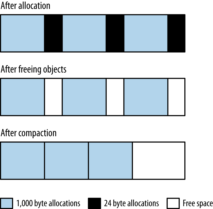
When the heap is full, the JVM will free the unused arrays. Say that all the 24-byte arrays are no longer in use, and the 1,000-byte arrays are still all in use: that yields the second row in Figure 5-1. The heap has free areas within it, but it can’t actually allocate anything larger than 24 bytes—unless the JVM moves all the 1,000-byte arrays so that they are contiguous, leaving all the free memory in a region where it can be allocated as needed (the third row in Figure 5-1).
The implementations are a little more detailed, but the performance of garbage collection is dominated by these basic operations: finding unused objects, making their memory available, and compacting the heap. Different collectors take different approaches to these operations, which is why they yield different performance characteristics.
It is simpler to perform these operations if no application threads are running while the garbage collector is running. Java programs are typically heavily multi-threaded, and the garbage collector itself often runs multiple threads. This discussion considers two logical groups of threads: the ones performing application logic, and the ones performing GC. When GC tracks object references, or moves objects around in memory, it must make sure that application threads are not using those objects. This is particularly true when GC moves objects around—the memory location of the object changes during that operation, and hence no application threads can be accessing the object.
The pauses when all application threads are stopped are called stop-the-world pauses. These pauses generally have the greatest impact on the performance of an application, and minimizing those pauses is the key consideration when tuning GC.
Generational Garbage Collectors
Though the details differ somewhat, all garbage collectors work by splitting the heap into different generations. These are called the old (or tenured) generation, and the young generation. The young generation is further divided into sections known as eden and the survivor spaces (though sometimes, eden is incorrectly used to refer to the entire young generation).
The rational for having separate generations is that many objects are used for a very short period of time. Take, for example, the loop in the stock price calculation where it sums the square of the difference of price from the average price (part of the calculation of standard deviation):
sum=newBigDecimal(0);for(StockPricesp:prices.values()){BigDecimaldiff=sp.getClosingPrice().subtract(averagePrice);diff=diff.multiply(diff);sum=sum.add(diff);}
Like many Java classes, the
BigDecimal
class is
immutable: the object represents a particular number and cannot be changed.
When arithmetic is performed on the object, a new object is created (and often,
the previous object with the previous value is then discarded). When
this simple loop is executed for a year’s worth of stock prices
(roughly 250 iterations),
750
BigDecimal
objects are created to store the intermediate
values just in this loop. Those objects are discarded on the next iteration of
the loop. Within the
add()
and other methods, the JDK library code creates even more
intermediate
BigDecimal
(and other) objects. In the end, a lot of objects
are created and discarded very quickly in this very small amount of code.
This kind of operation is quite common in Java, and so the garbage collector is designed to take advantage of the fact that many (and sometimes most) objects are only used temporarily. This is where the generational design comes in. Objects are first allocated in the young generation, which is some subset of the entire heap. When the young generation fills up, the garbage collector will stop all the application threads and empty out the young generation. Objects that are no longer in use are discarded, and objects that are still in use are moved elsewhere. This operation is called a minor GC.
There are two performance advantages to this design. First, because the young generation is only a portion of the entire heap, processing it is faster than processing the entire heap. This means that the application threads are stopped for a much shorter period of time than if the entire heap were processed at once. You probably see a trade-off there, since it also means that the application threads are stopped more frequently than they would be if the JVM waited to perform GC until the entire heap were full; that trade-off will be explored in more detail later in this chapter. For now, though, it is almost always a big advantage to have the shorter pauses even though they will be more frequent.
The second advantage arises from the way objects are allocated in the young generation. Objects are allocated in eden (which comprises the vast majority of the young generation). When the young generation is cleared during a collection, all objects in eden are either moved or discarded: all live objects are moved either to one of the survivor spaces or to the old generation. Since all objects are moved, the young generation is automatically compacted when it is collected.
All GC algorithms have stop-the-world pauses during collection of the young generation.
As objects are moved to the old generation, eventually it too will fill up, and the JVM will need to find any objects within the old generation that are no longer in use and discard those objects. This is the area where GC algorithms have their biggest differences. The simpler algorithms stop all application threads, find the unused objects and free their memory, and then compact the heap. This process is called a full GC, and it generally causes a long pause for the application threads.
On the other hand, it is possible—though more computationally complex—to find unused objects while application threads are running; CMS and G1 both take that approach. Because the phase where they scan for unused objects can occur without stopping application threads, CMS and G1 are called concurrent collectors. They are also called low-pause (and sometimes—incorrectly—pauseless) collectors, since they minimize the need to stop all the application threads. Concurrent collectors also take different approaches to compacting the old generation.
When using the CMS or G1 collector, an application will typically experience fewer (and much shorter) pauses. The trade-off is that the application will use more CPU overall. CMS and G1 may also perform a long, full GC pause (and avoiding those is one of the key factors to consider when tuning those algorithms).
As you consider which garbage collector is appropriate for your situation, think about the overall performance goals that must be met. There are trade-offs in every situation. In an application (such as a Java EE server) measuring the response time of individual requests, consider these points:
- The individual requests will be impacted by pause times—and more importantly by long pause times for full GCs. If minimizing the effect of pauses on response times is the goal, a concurrent collector will be more appropriate.
- If the average response time is more important than the outliers (i.e., the 90th% response time), the throughput collector will usually yield better results.
- The benefit of avoiding long pause times with a concurrent collector comes at the expense of extra CPU usage.
Similarly, the choice of garbage collector in a batch application is guided by the following trade-off:
- If enough CPU is available, using the concurrent collector to avoid full GC pauses will allow the job to finish faster.
- If CPU is limited, then the extra CPU consumption of the concurrent collector will cause the batch job to take more time.
Quick Summary
- All GC algorithms divide the heap into old and young generations.
- All GC algorithms employ a stop-the-world approach to clearing objects from the young generation, which is usually a very quick operation.
GC Algorithms
The JVM provides four different algorithms for performing GC.
The Serial Garbage Collector
The simplest of the garbage collectors is the serial garbage collector. This is the default collector if the application is running on a client-class machine (32-bit JVMs on Windows or on single-processor machines).
The serial collector uses a single thread to process the heap. It will stop all application threads as the heap is processed (for either a minor or full GC). During a full GC, it will fully compact the old generation.
The serial collector is
enabled by using the
-XX:+UseSerialGC
flag (though usually it is the default in those cases where it might be used).
Note that
unlike most JVM flags, the serial collector is not disabled changing the plus
sign to a minus sign (i.e., by specifying
-XX:-UseSerialGC).
On systems where the serial collector is the default,
it is disabled by specifying a different GC algorithm.
The Throughput Collector
This is the default collector for server class machines (multi-CPU Unix machines, and any 64-bit JVM).
The throughput collector
uses multiple threads to collect the young generation, which makes
minor GCs much faster than when the serial collector is used.
The throughput collector can use multiple threads to process the old
generation as well. That is the default behavior in JDK 7u4 and later
releases, and that behavior can be enabled in earlier JDK 7 JVMs
by specifying the
-XX:+UseParallelOldGC
flag. Because it uses multiple
threads, the throughput collector is often called the parallel collector.
The throughput collector stops all application threads during both minor
and full GCs, and it fully compacts the old generation during a full GC.
Since it is the default in most situations where it would be used, it
needn’t be explicitly enabled. To enable it where necessary, use
the flags
-XX:+UseParallelGC
-XX:+UseParallelOldGC.
The CMS Collector
The CMS collector is designed to eliminate the long pauses associated with
the full GC cycles of the throughput and serial collectors. CMS
stops all application
threads during a minor GC, which it also performs with multiple threads.
Notably, though, CMS uses a different algorithm to collect the young
generation
(-XX:+UseParNewGC)
than the throughput collector uses
(-XX:+UseParallelGC).
Instead of stopping the application threads during a full GC, CMS uses one or more background threads to periodically scan through the old generation and discard unused objects. This makes CMS a low-pause collector: application threads are only paused during minor collections, and for some very short periods of time at certain points as the background threads scan the old generation. The overall amount of time that application threads are stopped is much less than with the throughput collector.
The trade-off here comes with increased CPU usage: there must be adequate CPU available for the background GC thread(s) to scan the heap at the same time the application threads are running. In addition, the background threads do not perform any compaction, which means that the heap can become fragmented. If the CMS background threads don’t get enough CPU to complete their tasks, or if the heap becomes too fragmented to allocate an object, CMS reverts to the behavior of the serial collector: it stops all application threads in order to clean and compact the old generation using a single thread. Then it begins its concurrent, background processing again (until, possibly, the next time the heap becomes too fragmented).
CMS is enabled by specifying the flags
-XX:+UseConcMarkSweepGC
-XX:+UseParNewGC
(both of which are false by default).
The G1 Collector
The G1 (or Garbage First) collector is designed to process large heaps (greater than about 4 GB) with minimal pauses. It divides the heap into a number of regions, but it is still a generational collector. Some number of those regions comprise the young generation, and the young generation is still collected by stopping all application threads and moving all objects that are alive into the old generation or the survivor spaces. As in the other algorithms, this occurs using multiple threads.
G1 is a concurrent collector: the old generation is processed by background threads that don’t need to stop the application threads to perform most of their work. Because the old generation is divided into regions, G1 can clean up objects from the old generation by copying from one region in to another, which means that it (at least partially) compacts the heap during normal processing. Hence, a G1 heap is much less likely to be subject to fragmentation—though that is still possible.
Like CMS, the trade-off for avoiding the full GC cycles is CPU time:
the multiple background threads
must have CPU cycles available at the same time the application threads are
running.
G1 is enabled by specifying the
flag
-XX:+UseG1GC
(which by default is false).
Quick Summary
- The four available GC algorithms take different approaches towards minimizing the effect of GC on an application.
- The serial collector makes sense (and is the default) when only one CPU is available and extra GC threads would interfere with the application.
- The throughput collector is the default on other machines; it maximizes the total throughput of an application but may subject individual operations to long pauses.
- The CMS collector can collect the old generation concurrently with application threads still run. If enough CPU is available for its background processing, this can avoid full GC cycles for the application.
- The G1 collector also collects the old generation concurrently with application threads, potentially avoiding full GCs. Its design makes it less like to experience full GCs than CMS.
Choosing a GC Algorithm
The choice of a GC algorithm depends in part what the application looks like, and in part on the performance goals for the application.
The serial collector is best used only in those cases where the the application uses less than 100 MB. That allows the application to request a small heap, one that isn’t going to be helped by the parallel collections of the throughput collector, nor by the background collections of CMS or G1.
That sizing guideline limits the usefulness of the serial collector. Most programs will need to choose between the throughput collector and a concurrent collector; that choice is most influenced by the performance goals of the application.
An overview of this topic was discussed in Chapter 2: there is a difference in measuring an application’s elapsed time, throughput, or average (or 90th%) response times.
GC Algorithms and Batch Jobs
For batch jobs, the pauses introduced by the throughput collector—and particularly the pauses of the full GC cycles—are a big concern. Each one adds a certain amount of elapsed time to the overall execution time. If each full GC cycle takes 0.5 seconds and there are 20 such cycles during the five-minute execution of a program, then the pauses have added a 3.4% performance penalty: without the pauses, the program would have completed in 290 rather than 300 seconds.
If extra CPU is available (and that might be a big if), then using a concurrent collector will give the application a nice performance boost. The key here is whether adequate CPU is available for the background processing of the concurrent GC threads. Take the simple case of a single-CPU machine where there is a single application thread that consumes 100% of the CPU. When that application is run with the throughput collector, then GC will periodically run, causing the application thread to pause. When the same application is run with a concurrent collector, the operating system will sometimes run the application thread on the CPU, and sometimes run the background GC thread. The net effect is the same: the application thread is effectively paused (albeit for much shorter times) while the OS is running other threads.
The same principle applies in the general case when there are multiple application threads, multiple background GC threads, and multiple CPUs. If the operating system can’t run all the application threads at the same time as the background GC threads, then the competition for the CPU has effectively introduced pauses into the behavior of the application threads.
Table 5-1 shows how this trade-off works. The batch application calculating stock data has been run in a mode that saves each set results in memory for a few minutes (to fill up the heap); the test was run with a CMS and throughput GC algorithm.
| GC Algorithm | 4 CPUs (CPU utilization) | 1 CPU (CPU utilization) |
CMS | 78.09 (30.7%) | 120.0 (100%) |
Throughput | 81.00 (27.7%) | 111.6 (100%) |
The times in this table are the number of seconds required to run the test, and the CPU utilization of the machine is shown in parenthesis. When four CPUs are available, CMS runs a batch of operations about three seconds faster than the throughput collector—but notice the amount of CPU utilized in each case. There is a single application thread which will continually run, so with four CPUs, that application thread will consume 25% of the available CPU.
The extra CPU reported in the table comes from the extra processing introduced by the GC threads. In the case of CMS, the background thread periodically consumes an entire CPU, or 25% of the total CPU available on the machine. The background thread here runs periodically—it turned out to run about 5% of the time—leaving an average CPU utilization of 30%.
Similarly, the throughput collector runs four garbage collection threads. During GC cycles, those threads consume 100% of the four available CPUs, leaving a 28% average usage during the entire test. During minor collections, CMS will also run four GC threads that consume 100% of the four CPUs.
When only a single CPU is available, the CPU is always busy—whether running the application or GC threads. Now the extra overhead of the CMS background thread is a drawback, and the throughput collector finishes nine seconds sooner.
Looking at only the average CPU during a test misses the interesting picture of what happens during GC cycles. The throughput collector will (by default) consume 100% of CPU available on the machine while it runs, so a more accurate representation of the CPU usage during this test is shown in Figure 5-2.
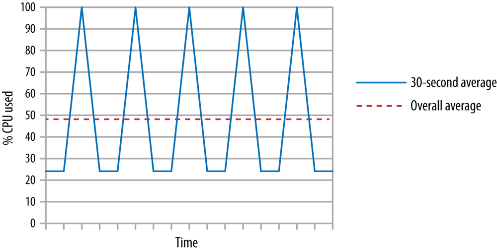
Most of the time, only the application thread is running, consuming 25% of total cpu. When GC kicks in, 100% of CPU is consumed. Hence, the actual CPU usage resembles the saw-tooth pattern in the graph, even though the average during the test is reported as the value of the straight dashed line.
The effect is different in a concurrent collector, when there are background thread(s) running concurrently with the application threads. In that case, a graph of the CPU might look like Figure 5-3.

The application thread starts by using 25% of total CPU. Eventually it has created enough garbage for the CMS background thread to kick in; that thread also consumes an entire CPU bringing the total up to 50%. When the CMS thread finishes, CPU usage drops to 25%, and so on. Note that there are no 100% peak CPU periods, which is a little bit of a simplification: there will be very short spikes to 100% CPU usage during the CMS young generation collections, but those are short enough that we can ignore them for this discussion.
There can be multiple background threads in a concurrent collector, but the effect is similar: when those background threads run, they will consume CPU and drive up the long-term CPU average.
This can be quite important when you have a monitoring system triggered by CPU usage rules: you want to make sure CPU alerts are not triggered by the 100% CPU usage spikes in a full GC, or the much longer (but lower) spikes from background concurrent processing threads. These spikes are normal occurrences for Java programs.
Quick Summary
- Batch jobs with application threads that utilize most of the CPU will typically get better performance from the throughput collector.
- Batch jobs that do not consume all the available CPU on a machine will typically get better performance with a concurrent collector.
GC Algorithms and Throughput Tests
When a test measures throughput, the basic trade-offs in GC algorithms are the same as for batch jobs, but the effect of the pauses is quite different. The overall system impact on CPU still plays an important consideration.
This section uses the stock servlet as the basis for its testing; the servlet is run in a GlassFish instance with a 2 GB heap, and the previous 10 requests are saved in each user’s http session (to put more pressure on the GC system). Table 5-2 shows the throughput the test achieves when running with the throughput and CMS collectors. In this case, the tests are run on a machine with four CPUs.
| Number of Clients | Throughput TPS (CPU Usage) | CMS TPS (CPU Usage) |
1 | 30.43 (29%) | 31.98 (31%) |
10 | 81.34 (97%) | 62.20 (85%) |
Two tests are run to measure the total throughput. In the first test,
a single client is emulated by the fhb program; the second cases drives
the load from 10 clients so that the target machine CPU is fully utilized.
When there are available CPU cycles, CMS performs better here, yielding 5% more TPS than the throughput collector. The throughput collector in this test had 24 full GC pauses during which it could not process requests; those pauses were about 5% of the total steady state time of the test. By avoiding those pauses, CMS provided better throughput.
When CPU was limited, however, CMS performed much worse: about 23.5% fewer TPS. Note too that CMS could not keep the CPU close to 100% busy in this experiment. That’s because there were not sufficient CPU cycles for the background CMS threads, and so CMS encountered concurrent mode failures. Those failures meant the JVM had to perform a single-threaded full GC, and those periods of time (during which the four-CPU machine was only 25% busy) drove down the average CPU utilization.
GC Algorithms and Response Time Tests
Table 5-3 shows the same test with a think time of 250 milliseconds between requests, which results in a fixed load of 29 TPS. The performance measurement then is the average, 90th%, and 99th% response times for each request.
| Session Size | Throughput Avg/90th%/99th% (CPU) | CMS Avg/90th%/99th% (CPU) |
10 items | 0.092/0.171/0.813 (41%) | 0.104/0.211/0.260 (46%) |
50 items | 0.180/0.218/3.617 (55%) | 0.107/0.222/0.315 (53%) |
The first test uses the parameter for saving the session state: the previous 10 requests are saved. The result here is typical when comparing the two collectors: the throughput collector is faster than the concurrent collector in terms of an average response time and even the 90th% response time. The 99th% response time shows a significant advantage for CMS: the full GCs in the throughput case made 1% of the operations (those that were stopped during a full GC) take significantly longer. CMS uses about 10% more CPU to get that improvement in the 99th% result.
When 50 items were saved in the session data, GC cycles had a much bigger impact—particularly in the throughput case. Now the average response time for the throughput collector is much higher than CMS, and all because of the very large outliers that drove the 99th% response time over three seconds. Interestingly, the 90th% response time for the throughput collector is lower than for CMS—when the JVM isn’t doing those full GCs, the throughput collector still shows an advantage.
Cases like that certainly occur from time to time, but they are far less common than the first case. In a sense, CMS was lucky in the last case too: often when the heap contains so much live data that the full GC time dominates the response times for the throughput collector, the CMS collector often experiences concurrent mode failures as well. In this example, the CMS background processing was sufficient to keep up with the demands of the application.
These are the sort of trade-offs to consider when deciding which GC algorithm suits your performance goals. If the average time is all you care about, then the throughput collector will likely look similar to a concurrent collector and you can consider the CPU usage instead (in which case, the throughput collector will be the better choice). If you’re interested in the 90th% or other percentile-based response times, then only testing can see where those line up with the number of full GC cycles the application needs to perform its job.
Quick Summary
- When measuring response time or throughput, the choice between throughput and concurrent collectors is dependent on the amount of CPU available for the background concurrent threads to run.
- The throughput collector will frequently have a lower average response time than a concurrent collector, but the concurrent collector will often have a lower 90th% or 99th% response time.
- When the throughput collector performs excessive full GCs, a concurrent collector will often have lower average response times.
Choosing between CMS and G1
The tests in the last section used CMS as the concurrent collector. As a basic rule of thumb, CMS is expected to outperform G1 for heaps that are smaller than 4 GB. CMS is a simpler algorithm than G1, and so in simple cases (i.e., those with small heaps), it is likely to be faster. When large heaps are used, G1 will usually be better than CMS because of the manner in which it can divide work.
CMS background thread(s) must scan the entire old generation before any objects can be freed. The time to scan the heap is obviously dependent on the size of the heap. If the CMS background thread does not finish scanning the heap and freeing objects before the heap fills up, CMS will experience a concurrent mode failure: at that point, CMS has to revert to doing a full GC with all application threads stopped. That full GC is done only with a single thread, making it a very severe performance penalty. CMS can be tuned to utilize multiple background threads to minimize that change, but the larger the heap grows, the more work those CMS threads have to do.[22]
G1, on the other hand, segments the old generation into regions, so it is easier for multiple background threads to divide the necessary work of scanning the old generation. G1 can still experience concurrent mode failures if the background threads can’t keep up, but the G1 algorithm makes that less likely to occur.
CMS can also revert to a full GC because of heap fragmentation, since CMS does not compact the heap (except during the lengthy full GCs). G1 compacts the heap as it goes. G1 can still experience heap fragmentation, but its design again reduces the change of that compared to CMS.
There are ways to tune both CMS and G1 to attempt to avoid these failures, but for some applications, that will not always work. As heaps grow larger (and the penalty for a full GC grows larger), it is easier to use G1 to avoid these issues.[23]
Finally, there are some slightly intangible factors to consider between all three collectors. The throughput collector is the oldest of the three collectors, which means the JVM engineers have had more opportunity to make sure that it is written to perform well in the first place. G1, as a relatively new algorithm, is more likely to encounter corner cases which its design didn’t anticipate. G1 has fewer tuning knobs to affect its performance, which may be good or bad depending on your perspective. G1 was considered experimental until Java 7u4, and some tuning features discussed later in this chapter aren’t available until Java 7u10. G1 has significant performance benefits in Java 8 and Java 7u60 compared to earlier Java 7 releases. Future work on G1 can also be expected to improve its performance on smaller heaps relative to CMS.
Quick Summary
- CMS is the better of the concurrent collectors when the heap is small.
- G1 is designed to process the heap is regions so it will scale better than CMS on large heaps.
Basic GC Tuning
Although GC algorithms differ in the way the process the heap, they share basic configuration parameters. In many cases, these basic configurations are all that is needed to run an application.
Sizing the Heap
The first basic tuning for GC is the size of the application’s heap. There are advanced tunings that affect the size of the heap’s generations; as a first step, this section will discuss setting the overall heap size.
Like most performance issues, choosing a heap size is a matter of balance. If the heap is too small, the program will spend too much time performing GC and not enough time performing application logic. But simply specifying a very large heap isn’t necessarily the answer either. The time spent in GC pauses is dependent on the size of the heap, so as the size of the heap increases, the duration of those pauses also increases. The pauses will occur less frequently, but their duration will make the overall performance lag.
A second danger arises when very large heaps are used. Computer operating systems use virtual memory to manage the physical memory of the machine. A machine may have 8 GB of physical RAM, but the OS will make it appear as if there is much more memory available. The amount of virtual memory is subject to the OS configuration, but say the OS makes it look like there is 16 GB of memory. The OS manages that by a process called swapping.[24] You can load programs that use up to 16 GB of memory, and the OS will copy inactive portions of those programs to disk. When those memory areas are needed, the OS will copy them from disk to RAM (and usually, it will first need to copy something from RAM to disk to make room).
This process works well for a system running lots of different applications, since most of the applications are not active at the same time. It does not work so well for Java applications. If a Java program with a 12 GB heap is run on this system, the OS can handle it by keeping 8 GB of the heap in RAM and 4 GB on disk (that simplifies the actual situation a little, since other programs will use part of RAM). The JVM won’t know about this; the swapping is transparently handled by the OS. Hence, the JVM will happily fill up all 12GB of heap it has been told to use. This causes a severe performance penalty as the OS swaps data from disk to RAM (which is an expensive operation to begin with).
Worse, the one time this swapping is guaranteed to occur is during a full GC, when the JVM must access the entire heap. If the system is swapping during a full GC, pauses will be an order of magnitude longer than they would otherwise be. Similarly, if a concurrent collector is used, when the background thread sweeps through the heap, it will likely fall behind due to the long waits for data to be copied from disk to main memory—resulting in an expensive concurrent mode failure.
Hence, the first rule is sizing a heap is never to specify a heap that is larger than the amount of physical memory on the machine—and if there are multiple JVMs running, that applies to the sum of all their heaps. You also need to leave some room for the JVM itself as well as some memory for other applications—typically, at least 1GB of space for common OS profiles.
The size of the heap is controlled by two values: an initial value
(specified with
-XmsN)
and a maximum value
(-XmxN).
The defaults for
these vary depending on the operating system, the amount of system RAM,
and the JVM in use. The defaults can also be affected by other flags on the
command line as well; heap sizing is one of the JVM’s core ergonomic tunings.
The goal of the JVM is to find a “reasonable” default initial value for the heap based on the system resources available to it, and to grow the heap up to a “reasonable” maximum if (and only if) the application needs more memory (based on how much time it spends performing GC). Absent some of the advanced tunings flags and details discussed later in this and the next chapters, the default values for the initial and maximum sizes are given in Table 5-4.[25]
| Operating System and JVM | Initial Heap (Xms) | Maximum Heap (Xmx) |
Linux/Solaris, 32-bit Client | 16 MB | 256 MB |
Linux/Solaris, 32-bit Server | 64 MB | MIN(1 GB, 1/4 of Physical Memory) |
Linux/Solaris, 64-bit Server | MIN(512MB, 1/64 of Physical Memory) | MIN(32GB, 1/4 of Physical Memory) |
MacOS 64-bit Server JVMs | 64 MB | MIN(1 GB, 1/4 of Physical Memory) |
Windows 32-bit Client JVMs | 16 MB | 256MB |
Windows 64-bit ServerJVMs | 64 MB | MIN(1 GB, 1/4 of Physical Memory) |
On a machine with less than 192MB of physical memory, the maximum heap size will be half of the physical memory (96MB or less).
Having an initial and maximum size for the heap allows the JVM to tune its behavior depending on the workload. If the JVM sees that it is doing too much GC with the initial heap size, it will continually increase the heap until the JVM is doing the “correct” amount of GC, or until the heap hits its maximum size.
For many applications, that means a heap size doesn’t need to set at all. Instead, you specify the performance goals for the GC algorithm: the pause times you are willing to tolerate, the percentage of time you want to spend in GC, and so on. The details of that will depend on the GC algorithm used and are discussed in the next chapter (though even then, the defaults are chosen such that for a wide range of applications, those values needn’t be tuned either).
That approach usually works fine if an application does not need a larger
heap than the default maximum for the platform it is running on.
However, if the application is
spending too much time in GC, then the heap
size will need to be increased by setting the
-Xmx
flag. There is no
hard-and-fast rule on what size to choose (other than not specifying a size
larger than the machine can support). A good
rule of thumb is to size the heap so that it is 30% occupied after a full
GC. To calculate this, run the application until it has reached a
steady-state configuration: a point at which it has loaded anything it caches,
has created a maximum number of client connections, and so on. Then connect
to the application with
jconsole
force a full GC
and observe how much memory is used when the full GC completes.[26]
Be aware that the automatic sizing of the heap occurs even if you explicitly set the maximum size: the heap will start at its default initial size, and the JVM will grow the heap in order to meet the performance goals of the GC algorithm. There isn’t necessarily a memory penalty for specifying a larger heap than is needed: it will only grow enough to meet the GC performance goals.
On the other hand, if you know exactly what size heap the application needs,
then you
may as well set both the initial and maximum values of the heap to that
value (e.g.,
-Xms4096m
-Xmx4096m).
That makes GC slightly more efficient,
because it never needs to figure out whether the heap should be resized.
Quick Summary
- The JVM will attempt to find a reasonable minimum and maximum heap size based on the machine it is running on.
- Unless the application needs a larger heap than the default, consider tuning the performance goals of a GC algorithm (given in the next chapter) rather than fine-tuning the heap size.
Sizing the Generations
Once the heap size has been determined, you (or the JVM) must decide how much of the heap to allocate to the young generation, and how much to allocate to the old generation. The performance implication of this should be clear: if there is a relatively larger young generation, then it will be collected less often, and fewer objects will be promoted into the old generation. But on the other hand, because the old generation is relatively smaller, it will fill up more frequently and do more full GCs. Striking a balance here is the key.
Different GC algorithms attempt to strike this balance in a different way. However, all GC algorithms use the same set of flags to set the sizes of the generations; this section covers those common flags.
The command-line flags to tune the generation sizes all adjust the size of the young generation; the old generation gets everything that is left over. There are a variety of flags that can be used to size the young generation:
-
-XX:NewRatio=N - Set the ratio of the young generation to the old generation.
-
-XX:NewSize=N - Set the initial size of the young generation.
-
-XX:MaxNewSize=N - Set the maximum size of the young generation.
-
-XmnN -
Shorthand for setting both
NewSizeandMaxNewSizeto the same value.
The young generation is first sized by the
NewRatio,
which has a default
value of 2. Parameters that affect the sizing of heap spaces are generally
specified as as ratios; the value is used in an equation to determine the
percentage of space affected. The
NewRatio
value is used
in this formula:
Initial Young Gen Size = Initial Heap Size / (1 + NewRatio)
Plugging in the initial size of the
heap and the
NewRatio
yields the value that becomes the setting
for the young generation. By default, then, the young generation starts
out at 33% of the initial heap size.
Alternately, the size of the young generation can be set explicitly by
specifying
the
NewSize
flag. If that option is set, it will take precedence
over the value calculated from the
NewRatio,
There is no default for this flag (though
PrintFlagsFinal
will report a value of 1 MB).
If the flag isn’t set, the initial young generation size will be based
on the
NewRatio
calculation.
As the heap expands, the young generation size will expand as well, up to
the maximum size specified by the
MaxNewSize
flag. By default, that
maximum is also set using the
NewRatio
value, though it is based on
the maximum (rather than initial) heap size.
Tuning the young generation by specifying a range for its minimum and maximum
sizes ends up being fairly difficult. When a heap size is fixed
(by setting
-Xms
equal to
-Xmx),
it is usually preferable to use
-Xmn
to specify a fixed
size for the young generation as well. If an application needs a
dynamically-sized heap
and requires a larger (or smaller) young generation, then focus on setting
the
NewRatio
value.
Quick Summary
- Within the overall heap size, the sizes of the generations are controlled by how much space is allocated to the young generation.
- The young generation will grow in tandem with the overall heap size, but it can also fluctuate as a percentage of the total heap (based on the initial and maximum size of the young generation).
Sizing PermGen and Metaspace
When the JVM loads classes, it must keep track of certain metadata about those classes. From the perspective of an end-user, this is all just bookkeeping information. This data is held in a separate heap space. In Java 7, this is called the permgen (or permanent generation), and in Java 8, this is called the metaspace.
Permgen and metaspace are not exactly the same thing. In Java 7, permgen contains some miscellaneous objects that are unrelated to class data; these are moved into the regular heap in Java 8. Java 8 also fundamentally changes the kind of metadata that is held in this special region—though since end users don’t know what that data is in the first place, that change doesn’t really affect us. As an end user, all we need to know is that permgen/metaspace holds a bunch of class-related data, and that there are certain circumstances where the size of that region needs to be tuned.
Note that
permgen/metaspace does not hold the actual instance of the class (the
Class
objects),
nor reflection objects (e.g.,
Method
objects); those are held in the regular
heap. Information in permgen/metaspace is really only used by the compiler and
JVM runtime, and the data it holds is referred to as class metadata.
There isn’t a good way to calculate in advance how much space a particular program needs for its permgen/metaspace. The size will be proportional to the number of classes it uses, so bigger applications will need bigger areas. One of the advantages to phasing out permgen is that the metaspace rarely needs to be sized—because (unlike permgen), metaspace will by default use as much space as it needs. Table 5-5 lists the default initial and maximum sizes for permgen and metaspace.
| Default Initial Size | Default Maximum Permgen Size | Default Maximum Metaspace Size | |
32-bit Client JVM | 12 MB | 64 MB | Unlimited |
32-bit Server JVM | 16 MB | 64 MB | Unlimited |
64-bit JVM | 20.75 MB | 82 MB | Unlimited |
These memory regions behave just like a separate instance of the regular heap.
They are sized dynamically based on
an initial size and will increase as needed to
a maximum size. For permgen, the sizes are specified via these flags:
-XX:PermSize=N
and
-XX:MaxPermSize=N. Metaspace is sized with these flags:
-XX:MetaspaceSize=N
and
-XX:MaxMetaspaceSize=N.
Resizing these regions requires a full GC, so it is an expensive operation. If there are a lot of full GCs during the startup of a program (as it is loading classes), it is often because permgen or metaspace is being resized, so increasing the initial size is a good idea to improve startup in that case. Java 7 applications that define a lot of classes should increase the maximum size as well. Application servers, for example, typically specify a maximum permgen size of 128 MB, 192 MB, or more.
Contrary to its name, data stored in permgen is not permanent (metaspace, then, is a much better name). In particular, classes can be eligible for GC just like anything else. This is a very common occurrence in an application server, which creates new class loaders every time an application is deployed (or redeployed). The old class loaders are then unreferenced and eligible for GC, as are any classes which they defined. In a long development cycle in an application server, it is not unusual to see full GCs triggered during deployment: permgen or metaspace has filled up with the new class information, but the old class metadata can be freed.
Heap dumps (see Chapter 7) can be used to diagnose what classloaders exist,
which in turn can help determine if a classloader leak is filling up
permgen (or metaspace). Otherwise,
jmap can be used with the argument
-permstat
(in Java 7) or
-clstats
(in Java 8) to
print out information
about the class loaders. That particular command isn’t the most stable,
though, and it
cannot be recommended.
Quick Summary
- The permanent generation or metaspace holds class metadata (not class data itself). It behaves like a separate heap.
- For typical applications that do not load classes after startup, the initial size of this region can be based on its usage after all classes have been loaded. That will slightly speed up startup.
- Application servers doing development (or any environment where classes are frequently redefined) will see an occasional full GC caused when permgen/metaspace fills up and old class metadata is discarded.
Controlling Parallelism
All GC algorithms except for the serial collector use multiple threads.
The number of these threads is controlled
by the
-XX:ParallelGCThreads=N
flag. The value of this flag
affects the number of threads used for the following operations:
-
Collection of the young generation when using
-XX:+UseParallelGC. -
Collection of the old generation when using
-XX:+UseParallelOldGC. -
Collection of the young generation when using
-XX:+UseParNewGC. -
Collection of the young generation when using
-XX:+UseG1GC. - Stop-the-world phases of CMS (though not full GCs).
- Stop-the-world phases of G1 (though not full GCs).
Because these GC operations stop the application threads from executing,
the JVM attempts to use as many CPU resources as it can in order to
minimize the pause time. By default, that means the JVM will run
one thread for each CPU on a machine, up to eight. Once
that threshold has been reached, the JVM only adds a new thread for every
5/8ths of a CPU. So the total number of threads (where N is the number
of CPUs on the machine) on a machine with more than eight CPUs is:
ParallelGCThreads = 8 + ((N - 8) * 5 / 8)
There are times when this number is too large. An application using a small heap (say, 1 GB) on a machine with eight CPUs will be slightly more efficient with four or six threads dividing up that heap. On a 128-CPU machine, 83 GC threads is too many for all but the largest heaps.
Additionally, if more than one JVM are running on the machine, it is a good idea to limit the total number of GC threads among all JVMs. When they run, the GC threads are quite efficient and each will consume 100% of a single CPU (this is why the CPU usage for the throughput collector was higher than expected in previous examples). In machines with eight or fewer CPUs, GC will consume 100% of the CPU on the machine. On machines with more CPUs and multiple JVMs, there will still be too many GC threads running in parallel.
Take the example of a 16-CPU machine running four JVMs; each JVM will have by default 13 GC threads. If all four JVMs execute GC at the same time, the machine will have 52 CPU-hungry threads contending for CPU time. That results in a fair amount of contention; it will be more efficient if each JVM is limited to four GC threads. Even though it may be unlikely for all four JVMs to perform a GC operation at the same time, one JVM executing GC with 13 threads means that the application threads in the remaining JVMs now have to compete for CPU resources on a machine where 13 of 16 CPUs are 100% busy executing GC tasks. Giving each JVM four GC threads provides a better balance in this case.
Note that this flag does not set the number of background threads used by CMS or G1 (though it does affect that). Details on that are given in the next chapter.
Quick Summary
- The basic number of threads used by all GC algorithms is based on the number of CPUs on a machine.
- When multiple JVMs are run on a single machine, that number will be too high and must be reduced.
Adaptive Sizing
The sizes of the heap, the generations, and the survivor spaces can vary during execution as the JVM attempts to find the optimal performance according to its policies and tunings.
This is a best-effort solution, and it relies on past performance: the assumption is that future GC cycles will look similar to the GC cycles in the recent past. That turns out to be a reasonable assumption for many workloads, and even if the allocation rate suddenly changes, the JVM will re-adapt its sizes based on the new information.
Adaptive sizing provides benefits in two important ways. First, it means that small applications don’t need to worry about over-specifying the size of their heap. Consider the administrative command-line programs used to adjust the operations of things like an application server—those programs are usually very short-lived and use minimal memory resources. These applications will use 16 (or 64) MB of heap even though the default heap could potentially grow to 1 GB. Because of adaptive sizing, applications like that don’t need to be specifically tuned; the platform defaults ensure that they will not use a large amount of memory.
Second, it means that many applications don’t really need to worry about tuning their heap size at all—or if they need a larger heap than the platform default, they can just specify that larger heap and forget about the other details. The JVM can auto-tune the heap and generation sizes to use an optimal amount of memory given the GC algorithm’s performance goals. Adaptive sizing is what allows that auto-tuning to work.
Still, doing the adjustment of the sizes takes a small amount of time—time which occurs for the most part during a GC pause. If you have taken the time to finely-tune GC parameters and the size constraints of the application’s heap, adaptive sizing can be disabled. Disabling adaptive sizing is also useful for applications that go through markedly different phases, and you want to optimally tune GC for one of those phases.
At a global level, adaptive sizing is disabled by turning off the
-XX:-UseAdaptiveSizePolicy
flag (which is true by default).
With the exception of the survivor spaces (which are examined in detail
in the next chapter), adaptive sizing is also effectively turned off if
the
minimum and maximum heap sizes are set to the same value,
and the initial and maximum sizes of the new generation are set to the
same value.
In order to see how the JVM is resizing the spaces in an application,
set the
-XX:+PrintAdaptiveSizePolicy
flag. When a GC is performed, the
GC log will contain information detailing how the various generations
were resized during a collection.
Quick Summary
- Adaptive sizing controls how the JVM alters the ratio of young generation to old generation within the heap.
- Adaptive sizing should generally be kept enabled, since adjusting those generation sizes is how GC algorithms attempt to meet their pause time goals.
- For finely-tuned heaps, adaptive sizing can be disabled for a small performance boost.
GC Tools
Since GC is central to the performance of Java, there are many tools that monitor its performance.
The best way to see what effect GC has on the performance of an application is to become familiar with the GC log, which is a record of every GC operation during the program’s execution.
The details in the GC log vary depending on the GC algorithm, but the basic management of the log is always the same. That management is covered here, and more details on the contents of the log are given in the algorithm-specific tuning sections in the next chapter.
There are multiple ways enable the GC log: specifying either of the flags
-verbose:gc
or
-XX:+PrintGC
will create a simple GC log (the flags are aliases for
each other, and by default the log is disabled).
The
-XX:+PrintGCDetails
flag will create a log
with much more information. This flag is recommended (it is also false
by default); it is often
too difficult to diagnose what is happening with GC using only the simple
log. In conjunction with the detailed log, it is recommended to include
-XX:+PrintGCTimeStamps
or
-XX:+PrintGCDateStamps,
so that the time between GC operations can be determined. The difference in
those two arguments is that the time stamps are relative to 0 (based on
when the JVM starts), while the date stamps are an actual date string.
That makes the date stamps ever-so-slightly less efficient as the dates are
formatted, though it is an infrequent enough operation that its effect is
unlikely to be noticed.
The GC log is written to standard output, though that location can be changed
with the
-Xloggc:path
flag. Using
Xloggc
automatically enables the simple GC log unless
PrintGCDetails
has also been enabled. The amount of data that is
kept in the GC log can be limited by using log rotation; this
is quite useful for a
long-running server that
might otherwise fill up its disk with logs over several months. Log file
rotation is controlled with these flags:
-XX:+UseGCLogFileRotation
-XX:NumberOfGCLogFiles=N
-XX:GCLogFileSize=N.
By default,
UseGCLogFileRotation
is disabled. When that flag is enabled, the default number
of files is 0 (meaning unlimited), and the default log file size is 0
(meaning unlimited).
Hence, values must be specified for all these options
in order for log rotation to work as expected. Note
that a log file size will be rounded up to 8K for values less than that.
You can parse and peruse the GC log files on your own. though there are several tools that do that. One of these is GC Histogram (http://java.net/projects/gchisto). GC Histogram reads in a GC log and provide several charts and tables about the data in that log. A summary of the overhead of GC produced by GC Histogram is shown in Figure 5-4.

In this particular case, the JVM is spending 41% (!) of time performing GC, and the time to perform a full GC is more than 7 seconds. This is an application that definitely needs to improve its memory usage.
For real-time monitoring of the heap, use jconsole. The Memory
panel of jconsole displays a real-time graph of the heap as shown in
Figure 5-5.
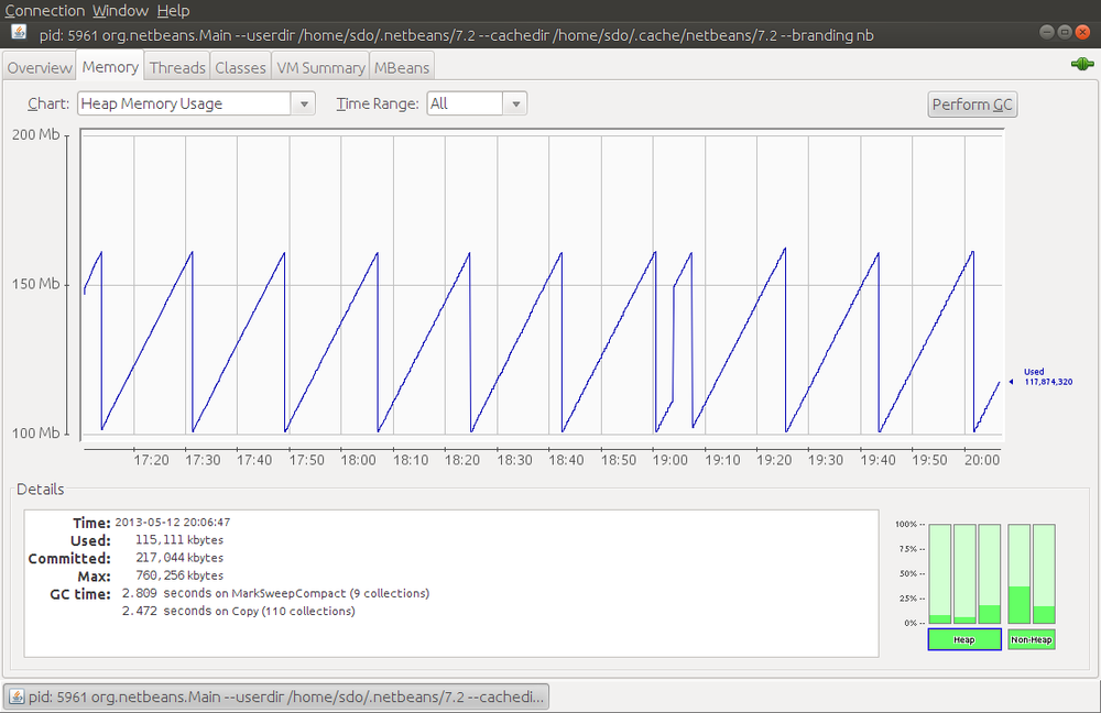
This particular view shows the entire heap, which is periodically
cycling between using about 100 MB and 160 MB. jconsole can instead
display only
eden, or the survivor spaces, or the old generation, or the permanent
generation. If I’d selected eden as the region to chart, it would have shown a
similar pattern
as eden fluctuated between 0 MB and 60 MB (and, as you can guess, that means
if I’d charted the old generation, it would have been essentially
a flat line at 100 MB).
For a scriptable solution,
jstat
is the tool of choice.
jstat
provides nine options to print different information about the heap;
jstat -options
will provide full list. One useful option
is
-gcutil,
which displays the time spent in GC as well as the percent
of each GC area that is currently filled. Other options to
jstat
will display
the GC sizes in terms of KB.
Remember that
jstat
takes an optional
argument—the number of milliseconds to repeat the command—so it can
monitor over time the effect of GC in an application. Here is some sample
output repeated every second:
% jstat -gcutil process_id 1000
  S0     S1     E      O      P     YGC     YGCT    FGC    FGCT     GCT
 51.71   0.00  99.12  60.00  99.93     98    1.985     8    2.397    4.382
  0.00  42.08   5.55  60.98  99.93     99    2.016     8    2.397    4.413
  0.00  42.08   6.32  60.98  99.93     99    2.016     8    2.397    4.413
  0.00  42.08  68.06  60.98  99.93     99    2.016     8    2.397    4.413
  0.00  42.08  82.27  60.98  99.93     99    2.016     8    2.397    4.413
  0.00  42.08  96.67  60.98  99.93     99    2.016     8    2.397    4.413
  0.00  42.08  99.30  60.98  99.93     99    2.016     8    2.397    4.413
 44.54   0.00   1.38  60.98  99.93    100    2.042     8    2.397    4.439
 44.54   0.00   1.91  60.98  99.93    100    2.042     8    2.397    4.439
When monitoring started, the program had already performed 98 collections
of the young generation (YGC) which took a total of 1.985 seconds (YGCT).
It had also performed eight full GCs (FGC) requiring 2.397 seconds (FGCT); hence
the total time in GC (GCT) was 4.382 seconds.
All three sections of the young generation are displayed here: the two
survivor spaces (S0 and S1) and eden (E). The monitoring started just as
eden was filling up (99.12% full), so in the next second there was a young
collection: eden reduced to 5.55% full, the survivor spaces switched places,
and a small amount of memory was promoted to the old generation (O), which
increased to using 60.98% of its space. As is typical, there is little or
no change in the permanent generation (P) since all necessary classes
have already been loaded by the application.
If you’ve forgotten to enable GC logging; this is a good substitute to watch how GC operates over time.
Quick Summary
- GC logs are the key piece of data required to diagnose GC issues; they should be collected routinely (even on production servers).
-
The better GC log file is obtained with the
PrintGCDetailsflag. - Programs to parse and understand GC logs are readily available; they are quite helpful in summarizing the data in the GC log.
-
jstatcan provide good visibility in GC for a live program.
Summary
Performance of the garbage collector is one key feature to the overall performance of any Java application. For many applications, though, the only tuning required is to select the appropriate GC algorithm and, if needed, to increase the heap size of the application. Adaptive sizing will then allow the JVM to auto-tune its behavior to provide good performance using the given heap.
More complex applications will require additional tuning, particularly for specific GC algorithms. If the simple GC settings in this chapter do not provide the performance an application requires, consult the tunings described in the next chapter.
[22] The chance that CMS experiences a concurrent mode failure also depends on the amount of allocation that the application does.
[23] On the other hand, for some applications it is impossible to tune either collector to avoid concurrent mode failures. Hence, even if the performance goals for an application seem to be inline with the goals of a concurrent collector, the throughput collector may still be the better choice.
[24] Or paging, though there is also a technical difference between those two terms which isn’t important for this discussion.
[25] The JVM will round these values down slightly for alignment purposes; the GC logs that print the sizes will show that the values are not exactly equal to the numbers in this table.
[26] Alternately, for throughput GC, you can consult the GC log if it is available.