In a relational database, we have the database itself, which is the outermost container that might correspond to a single application. The database contains tables. Tables have names and contain one or more columns, which also have names. When we add data to a table, we specify a value for every column defined; if we don’t have a value for a particular column, we use null. This new entry adds a row to the table, which we can later read if we know the row’s unique identifier (primary key), or by using a SQL statement that expresses some criteria that row might meet. If we want to update values in the table, we can update all of the rows or just some of them, depending on the filter we use in a “where” clause of our SQL statement.

For the purposes of learning Cassandra, it may be useful to suspend for a moment what you know from the relational world.

In this section, we’ll take a bottom-up approach to understanding Cassandra’s data model.

The simplest data store you would conceivably want to work with might be an array or list. It would look like Figure 3-1.

Figure 3-1. A list of values

If you persisted this list, you could query it later, but you would have to either examine each value in order to know what it represented, or always store each value in the same place in the list and then externally maintain documentation about which cell in the array holds which values. That would mean you might have to supply empty placeholder values (nulls) in order to keep the uniform size in case you didn’t have a value for an optional attribute (such as a fax number or apartment number). An array is a clearly useful data structure, but not semantically rich.

So we’d like to add a second dimension to this list: names to match the values. We’ll give names to each cell, and now we have a map structure, as shown in Figure 3-2.

Figure 3-2. A map of name/value pairs

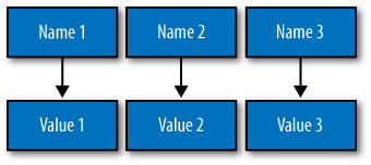
This is an improvement because we can know the names of our values. So if we decided that our map would hold User information, we could have column names like firstName, lastName, phone, email, and so on. This is a somewhat richer structure to work with.

But the structure we’ve built so far works only if we have one instance of a given entity, such as a single Person or User or Hotel or Tweet. It doesn’t give us much if we want to store multiple entities with the same structure, which is certainly what we want to do. There’s nothing to unify some collection of name/value pairs, and no way to repeat the same column names. So we need something that will group some of the column values together in a distinctly addressable group. We need a key to reference a group of columns that should be treated together as a set. We need rows. Then, if we get a single row, we can get all of the name/value pairs for a single entity at once, or just get the values for the names we’re interested in. We could call these name/value pairs columns. We could call each separate entity that holds some set of columns rows. And the unique identifier for each row could be called a row key.

Cassandra defines a column family to be a logical division that associates similar data. For example, we might have a User column family, a Hotel column family, an AddressBook column family, and so on. In this way, a column family is somewhat analogous to a table in the relational world.

Putting this all together, we have the basic Cassandra data structures: the column, which is a name/value pair (and a client-supplied timestamp of when it was last updated), and a column family, which is a container for rows that have similar, but not identical, column sets.

In relational databases, we’re used to storing column names as strings only—that’s all we’re allowed. But in Cassandra, we don’t have that limitation. Both row keys and column names can be strings, like relational column names, but they can also be long integers, UUIDs, or any kind of byte array. So there’s some variety to how your key names can be set.

This reveals another interesting quality to Cassandra’s columns: they don’t have to be as simple as predefined name/value pairs; you can store useful data in the key itself, not only in the value. This is somewhat common when creating indexes in Cassandra. But let’s not get ahead of ourselves.

Now we don’t need to store a value for every column every time we store a new entity. Maybe we don’t know the values for every column for a given entity. For example, some people have a second phone number and some don’t, and in an online form backed by Cassandra, there may be some fields that are optional and some that are required. That’s OK. Instead of storing null for those values we don’t know, which would waste space, we just won’t store that column at all for that row. So now we have a sparse, multidimensional array structure that looks like Figure 3-3.

Figure 3-3. A column family

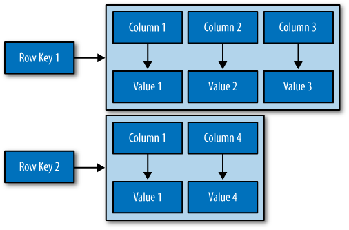
It may help to think of it in terms of JavaScript Object Notation (JSON) instead of a picture:

Musician:                         ColumnFamily 1
    bootsy:                       RowKey
        email: [email protected],  ColumnName:Value
        instrument: bass          ColumnName:Value
    george:                       RowKey
        email: [email protected]   ColumnName:Value

Band:                             ColumnFamily 2
    george:                       RowKey
        pfunk: 1968-2010          ColumnName:Value

Here we have two column families, Musician and Band. The Musician column family has two rows, “bootsy” and “george”. These two rows have a ragged set of columns associated with them: the bootsy record has two columns (email and instrument), and the george record has only one column. That’s fine in Cassandra. The second column family is Band, and it also has a “george” row, with a column named “pfunk”.

Columns in Cassandra actually have a third aspect: the timestamp, which records the last time the column was updated. This is not an automatic metadata property, however; clients have to provide the timestamp along with the value when they perform writes. You cannot query by the timestamp; it is used purely for conflict resolution on the server side.

And what if we wanted to create a group of related columns, that is, add another dimension on top of this? Cassandra allows us to do this with something called a super column family. A super column family can be thought of as a map of maps. The super column family is shown in Figure 3-4.

Figure 3-4. A super column family

Where a row in a column family holds a collection of name/value pairs, the super column family holds subcolumns, where subcolumns are named groups of columns. So the address of a value in a regular column family is a row key pointing to a column name pointing to a value, while the address of a value in a column family of type “super” is a row key pointing to a column name pointing to a subcolumn name pointing to a value. Put slightly differently, a row in a super column family still contains columns, each of which then contains subcolumns.

So that’s the bottom-up approach to looking at Cassandra’s data model. Now that we have this basic understanding, let’s switch gears and zoom out to a higher level, in order to take a top-down approach. There is so much confusion on this topic that it’s worth it to restate things in a different way in order to thoroughly understand the data model.

Cassandra is probably not the best choice if you only need to run a single node. As previously mentioned, the Cassandra database is specifically designed to be distributed over several machines operating together that appear as a single instance to the end user. So the outermost structure in Cassandra is the cluster, sometimes called the ring, because Cassandra assigns data to nodes in the cluster by arranging them in a ring.

A node holds a replica for different ranges of data. If the first node goes down, a replica can respond to queries. The peer-to-peer protocol allows the data to replicate across nodes in a manner transparent to the user, and the replication factor is the number of machines in your cluster that will receive copies of the same data. We’ll examine this in greater detail in Chapter 6.

A cluster is a container for keyspaces—typically a single keyspace. A keyspace is the outermost container for data in Cassandra, corresponding closely to a relational database. Like a relational database, a keyspace has a name and a set of attributes that define keyspace-wide behavior. Although people frequently advise that it’s a good idea to create a single keyspace per application, this doesn’t appear to have much practical basis. It’s certainly an acceptable practice, but it’s perfectly fine to create as many keyspaces as your application needs. Note, however, that you will probably run into trouble creating thousands of keyspaces per application.

Depending on your security constraints and partitioner, it’s fine to run multiple keyspaces on the same cluster. For example, if your application is called Twitter, you would probably have a cluster called Twitter-Cluster and a keyspace called Twitter. To my knowledge, there are currently no naming conventions in Cassandra for such items.

In Cassandra, the basic attributes that you can set per keyspace are:

I mention the replication factor and replica placement strategy here because they are set per keyspace. However, they don’t have an immediate impact on your data model per se.

It is possible, but generally not recommended, to create multiple keyspaces per application. The only time you would want to split your application into multiple keyspaces is if you wanted a different replication factor or replica placement strategy for some of the column families. For example, if you have some data that is of lower priority, you could put it in its own keyspace with a lower replication factor so that Cassandra doesn’t have to work as hard to replicate it. But this may be more complicated than it’s worth. It’s probably a better idea to start with one keyspace and see whether you really need to tune at that level.

A column family is a container for an ordered collection of rows, each of which is itself an ordered collection of columns. In the relational world, when you are physically creating your database from a model, you specify the name of the database (keyspace), the names of the tables (remotely similar to column families, but don’t get stuck on the idea that column families equal tables—they don’t), and then you define the names of the columns that will be in each table.

There are a few good reasons not to go too far with the idea that a column family is like a relational table. First, Cassandra is considered schema-free because although the column families are defined, the columns are not. You can freely add any column to any column family at any time, depending on your needs. Second, a column family has two attributes: a name and a comparator. The comparator value indicates how columns will be sorted when they are returned to you in a query—according to long, byte, UTF8, or other ordering.

In a relational database, it is frequently transparent to the user how tables are stored on disk, and it is rare to hear of recommendations about data modeling based on how the RDBMS might store tables on disk. That’s another reason to keep in mind that a column family is not a table. Because column families are each stored in separate files on disk, it’s important to keep related columns defined together in the same column family.

Another way that column families differ from relational tables is that relational tables define only columns, and the user supplies the values, which are the rows. But in Cassandra, a table can hold columns, or it can be defined as a super column family. The benefit of using a super column family is to allow for nesting.

For standard column families, which is the default, you set the type to Standard; for a super column family, you set the type to Super.

When you write data to a column family in Cassandra, you specify values for one or more columns. That collection of values together with a unique identifier is called a row. That row has a unique key, called the row key, which acts like the primary key unique identifier for that row. So while it’s not incorrect to call it column-oriented, or columnar, it might be easier to understand the model if you think of rows as containers for columns. This is also why some people refer to Cassandra column families as similar to a four-dimensional hash:

[Keyspace][ColumnFamily][Key][Column]

We can use a JSON-like notation to represent a Hotel column family, as shown here:

Hotel {
  key: AZC_043 { name: Cambria Suites Hayden, phone: 480-444-4444, 
    address: 400 N. Hayden Rd., city: Scottsdale, state: AZ, zip: 85255}
  key: AZS_011 { name: Clarion Scottsdale Peak, phone: 480-333-3333, 
    address: 3000 N. Scottsdale Rd, city: Scottsdale, state: AZ, zip: 85255} 
  key: CAS_021 { name: W Hotel, phone: 415-222-2222, 
    address: 181 3rd Street, city: San Francisco, state: CA, zip: 94103}
  key: NYN_042 { name: Waldorf Hotel, phone: 212-555-5555, 
    address: 301 Park Ave, city: New York, state: NY, zip: 10019}
}

In this example, the row key is a unique primary key for the hotel, and the columns are name, phone, address, city, state, and zip. Although these rows happen to define values for all of the same columns, you could easily have one row with 4 columns and another row in the same column family with 400 columns, and none of them would have to overlap.

We can query a column family such as this one using the CLI, like this:

cassandra> get Hotelier.Hotel['NYN_042']
=> (column=zip, value=10019, timestamp=3894166157031651)
=> (column=state, value=NY, timestamp=3894166157031651)
=> (column=phone, value=212-555-5555, timestamp=3894166157031651)
=> (column=name, value=The Waldorf=Astoria, timestamp=3894166157031651)
=> (column=city, value=New York, timestamp=3894166157031651)
=> (column=address, value=301 Park Ave, timestamp=3894166157031651)
Returned 6 results.

This indicates that we have one hotel in New York, New York, but we see six results because the results are column-oriented, and there are six columns for that row in the column family. Note that while there are six columns for that row, other rows might have more or fewer columns.

A column is the most basic unit of data structure in the Cassandra data model. A column is a triplet of a name, a value, and a clock, which you can think of as a timestamp for now. Again, although we’re familiar with the term “columns” from the relational world, it’s confusing to think of them in the same way in Cassandra. First of all, when designing a relational database, you specify the structure of the tables up front by assigning all of the columns in the table a name; later, when you write data, you’re simply supplying values for the predefined structure.

But in Cassandra, you don’t define the columns up front; you just define the column families you want in the keyspace, and then you can start writing data without defining the columns anywhere. That’s because in Cassandra, all of a column’s names are supplied by the client. This adds considerable flexibility to how your application works with data, and can allow it to evolve organically over time.

The data types for the name and value are Java byte arrays, frequently supplied as strings. Because the name and value are binary types, they can be of any length. The data type for the clock is an org.apache.cassandra.db.IClock, but for the 0.7 release, a timestamp still works to keep backward compatibility. This column structure is illustrated in Figure 3-5.

Figure 3-5. The structure of a column

Here’s an example of a column you might define, represented with JSON notation just for clarity of structure:

{
  "name": "email",
  "value: "[email protected]",
  "timestamp": 1274654183103300
}

In this example, this column is named “email”; more precisely, the value of its name attribute is “email”. But recall that a single column family will have multiple keys (or row keys) representing different rows that might also contain this column. This is why moving from the relational model is hard: we think of a relational table as holding the same set of columns for every row. But in Cassandra, a column family holds many rows, each of which may hold the same, or different, sets of columns.

On the server side, columns are immutable in order to prevent multithreading issues. The column is defined in Cassandra by the org.apache.cassandra.db.IColumn interface, which allows a variety of operations, including getting the value of the column as a byte array or, in the case of a super column, getting its subcolumns as a Collection<IColumn> and finding the time of the most recent change.

In a relational database, rows are stored together. This wasn’t the case for early versions of Cassandra, but as of version 0.6, rows for the same column family are stored together on disk.

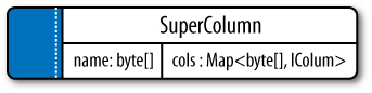
A super column is a special kind of column. Both kinds of columns are name/value pairs, but a regular column stores a byte array value, and the value of a super column is a map of subcolumns (which store byte array values). Note that they store only a map of columns; you cannot define a super column that stores a map of other super columns. So the super column idea goes only one level deep, but it can have an unbounded number of columns.

The basic structure of a super column is its name, which is a byte array (just as with a regular column), and the columns it stores (see Figure 3-6). Its columns are held as a map whose keys are the column names and whose values are the columns.

Figure 3-6. The basic structure of a super column

Each column family is stored on disk in its own separate file. So to optimize performance, it’s important to keep columns that you are likely to query together in the same column family, and a super column can be helpful for this.

The SuperColumn class implements both the IColumn and the IColumnContainer classes, both from the org.apache.cassandra.db package. The Thrift API is the underlying RPC serialization mechanism for performing remote operations on Cassandra. Because the Thrift API has no notion of inheritance, you will sometimes see the API refer to a ColumnOrSupercolumn type; when data structures use this type, you are expected to know whether your underlying column family is of type Super or Standard.

Here we see some more of the richness of the data model. When using regular columns, as we saw earlier, Cassandra looks like a four-dimensional hashtable. But for super columns, it becomes more like a five-dimensional hash:

[Keyspace][ColumnFamily][Key][SuperColumn][SubColumn]

To use a super column, you define your column family as type Super. Then, you still have row keys as you do in a regular column family, but you also reference the super column, which is simply a name that points to a list or map of regular columns (sometimes called the subcolumns).

Here is an example of a super column family definition called PointOfInterest. In the hotelier domain, a “point of interest” is a location near a hotel that travelers might like to visit, such as a park, museum, zoo, or tourist attraction:

PointOfInterest (SCF)
	SCkey: Cambria Suites Hayden
	{ 
		key: Phoenix Zoo 
		{
			phone: 480-555-9999,
			desc: They have animals here.
		},		
		key: Spring Training 
		{ 
			phone: 623-333-3333,
			desc: Fun for baseball fans.
			
		},
	}, //end of Cambria row 
	SCkey: (UTF8) Waldorf=Astoria
	{ 
		key: Central Park
			desc: Walk around. It's pretty.
		},		
		key: Empire State Building
		{ 
			phone: 212-777-7777,
			desc: Great view from the 102nd floor.
			
		}
	}
}

The PointOfInterest super column family has two super columns, each named for a different hotel (Cambria Suites Hayden and Waldorf=Astoria). The row keys are names of different points of interest, such as “Phoenix Zoo” and “Central Park”. Each row has columns for a description (the “desc” column); some of the rows have a phone number, and some don’t. Unlike relational tables, which group rows of identical structure, column families and super column families group merely similar records.

Using the CLI, we could query a super column family like this:

cassandra> get PointOfInterest['Central Park']['The Waldorf=Astoria']['desc']
=> (column=desc, value=Walk around in the park. It's pretty., timestamp=1281301988847)

This query is asking: in the PointOfInterest column family (which happens to be defined as type Super), use the row key “Central Park”; for the super column named “Waldorf=Astoria”, get me the value of the “desc” column (which is the plain language text describing the point of interest).

HotelByCity (CF) Key: city:state {
  key: Phoenix:AZ {AZC_043: -, AZS_011: -}
  key: San Francisco:CA {CAS_021: -}
  key: New York:NY {NYN_042: -}
}

There are several differences between Cassandra’s model and query methods compared to what’s available in RDBMS, and these are important to keep in mind.

SELECT hotelID FROM Hotel WHERE name = 'Clarion Midtown';

There are a few ways that people commonly use Cassandra that might be described as design patterns. I’ve given names to these common patterns: Materialized View, Valueless Column, and Aggregate Key.

Let’s look briefly at a few things to keep in mind when you’re trying to move from a relational mindset to Cassandra’s data model. I’ll just say it: if you have been working with relational databases for a long time, it’s not always easy. Here are a few pointers:

In this chapter we took a gentle approach to understanding Cassandra’s data model of keyspaces, column families, columns, and super columns. We also explored a few of the contrasts between RDBMS and Cassandra.