8 polar coordinates

In This Chapter

8.1 Polar Coordinates

8.2 Graphs of Polar Equations

8.3 Conic Sections in Polar Coordinates

      Chapter 8 Review Exercises

The sliced view of a nautilus shell shows an approximation to a curve called a logarithmic spiral. See Problem 31 in Exercises 8.2.

A Bit of History The rectangular or Cartesian coordinate system is one of many different coordinate systems that have been developed over the years to serve different purposes. In mathematical applications a problem that is intractable in rectangular coordinates may become tractable in a different coordinate system. In this chapter our primary study is of the polar coordinate system—a two-dimensional coordinate system in which points are specified by a directed distance from the origin and an angle measured from the positive x-axis.

Although bits and pieces of the concept of polar coordinates can be traced back to the Greek mathematicians Hipparchus (c. 190-120 BCE) and Archimedes (c. 287–212 BCE), the independent introduction of polar coordinates into the mathematical milieu of the seventeenth century is attributed to the Belgian Jesuit priest Grégoire de Saint–Vincent (1584–1667) and the Italian theologian and mathematician Bonaventura Cavalieri (1598–1647). However, it was the Italian mathematician Gregorio Fontana (1735–1803) who actually coined the term polar coordinates. This term appeared in English for the first time in the 1816 translation of Sylvestre François Lacroix' (French, 1765–1843) Differential and Integral Calculus by the English mathematician George Peacock (1791–1858).

8.1 Polar Coordinates

Introduction So far we have used the rectangular coordinate system to specify a point P in the plane. We can regard this system as a grid of horizontal and vertical lines. The coordinates (a, b) of a point P are determined by the intersection of two lines: one line x = a is perpendicular to the horizontal reference line called the x-axis, and the other y = b is perpendicular to the vertical reference line called the y-axis. See FIGURE 8.1.1(a). Another system for locating points in the plane is the polar coordinate system.

Terminology To set up a polar coordinate system, we use a system of circles centered at a point O, called the pole, and straight lines or rays emanating from O. We take as a reference axis a horizontal half-line directed to the right of the pole and call it the polar axis. By specifying a directed (signed) distance r from O and an angle θ whose initial side is the polar axis and whose terminal side is the ray OP, we label the point P by (r, θ). We say that the ordered pair (r, θ) are the polar coordinates of P. See Figures 8.1.1(b) and 8.1.1(c).

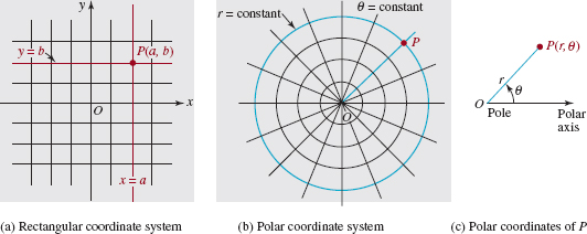
FIGURE 8.1.1 Comparison of rectangular and polar coordinates of a point P

Although the measure of the angle θ can be either in degrees or radians, in calculus radian measure is used almost exclusively. Consequently, we shall use only radian measure in this discussion.

In the polar coordinate system we adopt the following conventions.

EXAMPLE 1 Plotting Polar Points

Plot the points whose polar coordinates are given.

(a) (4, π/6)

(b) (2, –π/4)

(c) (–3, 3π/4)

Solution (a) Measure 4 units along the ray π/6 as shown in FIGURE 8.1.2(a).

(b) Measure 2 units along the ray -π/4. See FIGURE 8.1.2(b).

(c) Measure 3 units along the ray 3π/4 + π = 7π/4. Equivalently, we can measure 3 units along the ray 3π/4 extended backward through the pole. Note carefully in FIGURE 8.1.2(c) that the point (– 3, 3π/4) is not in the same quadrant as the terminal side of the given angle.

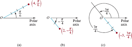
FIGURE 8.1.2 Points in polar coordinates in Example 1

In contrast to the rectangular coordinate system, the description of a point in polar coordinates is not unique. This is an immediate consequence of the fact that

                (r, θ) and (r, θ + 2nπ), n an integer,

are equivalent. To compound the problem, negative values of r can be used.

EXAMPLE 2 Equivalent Polar Points

The following coordinates are some alternative representations of the point (2, π/6):

(2, 13π/6), (2, –11π/6), (–2, 7π/6), (–2, –5π/6).

Conversion of Polar Coordinates to Rectangular By superimposing a rectangular coordinate system on a polar coordinate system, as shown in FIGURE 8.1.3, we can convert a polar description of a point to rectangular coordinates by using

These conversion formulas hold true for any values of r and θ in an equivalent polar representation of (r, θ).

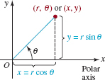
FIGURE 8.1.3 Relating polar and rectangular coordinates

EXAMPLE 3 Polar to Rectangular

Convert (2, π/6) in polar coordinates to rectangular coordinates.

Solution With r = 2, θ = π/6, we have from (1),

Thus, (2, π/6) is equivalent to (, 1) in rectangular coordinates.

Conversion of Rectangular Coordinates to Polar It should be evident from FIGURE 8.1.3 that x, y, r, and θ are also related by

The equations in (2) are used to convert the rectangular coordinates (x, y) to the polar coordinates (r, θ).

EXAMPLE 4 Rectangular to Polar

Convert (–1, 1) in rectangular coordinates to polar coordinates.

Solution With x = –1, y = 1, we have from (2)

r² = 2 and tanθ = –1.

Now, r² = 2 or r =±, and two of many angles that satisfy tanθ = –1 are 3π/4 and 7π/4. From FIGURE 8.1.4 we see that two polar representations for (–1, 1) are (, 3π/4) and (–, 7π/4).

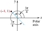
FIGURE 8.1.4 Point in Example 4

In Example 4, observe that we cannot pair just any angle θ and any value r that satisfy (2); these solutions must also be consistent with (1). Because the points (–, 3π/4) and (, 7π/4) lie in the fourth quadrant, they are not polar representations of the second-quadrant point (– 1, 1).

There are instances in calculus when a rectangular equation must be expressed as a polar equation r = f(θ). The next example shows how to do this using the conversion formulas in (1).

EXAMPLE 5 Rectangular Equation to Polar Equation

Find a polar equation that has the same graph as the circle x² + y² = 8x.

Solution Substituting x = rcosθ, y = rsinθ, into the given equation we find

The last equation implies that

r = 0   or   r = 8cosθ.

Since r = 0 determines only the pole O, we conclude that a polar equation of the circle is r = 8cosθ. Note that the circle x² + y² = 8x passes through the origin since x = 0 and y = 0 satisfy the equation. Relative to the polar equation r = 8cosθ of the circle, the origin or pole corresponds to the polar coordinates (0, π/2).

EXAMPLE 6 Rectangular Equation to Polar Equation

Find a polar equation that has the same graph as the parabola x² = 8(2 – y).

Solution We replace x and y in the given equation by x = rcosθ, y = rsinθ and solve for r in terms of θ:

Solving for r gives two equations,

Now recall that, by convention (ii) in Definition 8.1.1, (r, θ) and(–r, θ + π) represent the same point. You should verify that if (r, θ)is replaced by (–r, θ + π) in the second of these two equations, we obtain the first equation. In other words, the equations are equivalent and so we may simply take the polar equation of the parabola to be r = 4/(1 + sinθ).

EXAMPLE 7 Polar Equation to Rectangular Equation

Find a rectangular equation that has the same graph as the polar equation r² = 9cos2θ.

Solution First, we use the trigonometric identity for the cosine of a double angle:

Then, from r² = x² + y², cosθ = x/r, sinθ = y/r, we have

The next section will be devoted to graphing polar equations.

8.1 Exercises Answers to selected odd-numbered problems begin on page ANS-20.

In Problems 1-6, plot the point with the given polar coordinates.

 1. (3, π)

 2. (2, –π/2)

 3. (–, π/2)

 4. (–1, π/6)

 5. (–4, –π/6)

 6. (, 7π/4)

In Problems 7-12, find alternative polar coordinates that satisfy

 (a) r > 0, θ < 0

 (b) r > 0, θ > 2π

 (c) r < 0, θ > 0

 (d) r < 0, θ < 0

for each point with the given polar coordinates.

 7. (2, 3π/4)

 8. (5, π/2)

 9. (4, π/3)

 10. (3, π/4)

 11. (1, π/6)

 12. (3, 7π/6)

In Problems 13-18, find the rectangular coordinates for each point with the given polar coordinates.

 13. (, 2π/3)

 14. (– 1, 7π/4)

 15. (–6, –π/3)

 16. , 11π/6)

 17. (4, 5π/4)

 18. (–5, π/2)

In Problems 19-24, find polar coordinates that satisfy

 (a) r > 0, –π < θ ≤ π

 (b) r < 0, –π < θ ≤ π

for each point with the given rectangular coordinates.

 19. (–2, –2)

 20. (0, –4)

 21. (1, –)

 22. (, )

 23. (7, 0)

 24. (1, 2)

In Problems 25-30, sketch the region on the plane that consists of points (r, θ) whose polar coordinates satisfy the given conditions.

 25. 2 ≤ r < 4, 0 ≤ θ ≤ π

 26. 2 < r ≤ 4

 27. 0 ≤ r ≤ 2, -π/2 ≤ θ ≤ π/2

 28. r ≥ 0, π/4 < θ < 3π/4

 29. –1 ≤ r ≤ 1, 0 ≤ θ ≤ π/2

 30. –2 ≤ r < 4, π/3 ≤ θ ≤ π

In Problems 31-40, find a polar equation that has the same graph as the given rectangular equation.

 31. y = 5

 32. x + 1 = 0

 33. y = 7x

 34. 3x + 8y + 6 = 0

 35. y² = –4x + 4

 36. x² – 12y – 36 = 0

 37. x² + y² = 36

 38. x² – y² = 1

 39. x² + y² + x =

 40. x³ + y³ – xy = 0

In Problems 41-52, find a rectangular equation that has the same graph as the given polar equation.

 41. r = 2secθ

 42. rcosθ = –4

 43. r = 6sin2θ

 44. 2r = tanθ

 45. r² = 4sin2θ

 46. r²cos2θ = 16

 47. r + 5sinθ = 0

 48. r = 2 + cosθ

 49. r =

 50. r(4 – sinθ) = 10

 51. r =

 52. r = 3 + 3 secθ

For Discussion

 53. How would you express the distance d between two points (r₁, θ₁) and (r₂, θ₂) in terms of their polar coordinates?

 54. You know how to find a rectangular equation of a line through two points with rectangular coordinates. How would you find a polar equation of a line through two points with polar coordinates (r₁, θ₁) and (r₂, θ₂)? Carry out your ideas by finding a polar equation of the line through (3, 3π/4) and (1, π/4). Find the polar coordinates of the x- and y-intercepts of the line.

 54. In rectangular coordinates the x-intercepts of the graph of a function y = f(x) are determined from the solutions of the equation f(x) = 0. In the next section we will graph polar equations r = f(θ). What is the significance of the solutions of the equation f(θ) = 0?

8.2 Graphs of Polar Equations

Introduction The graph of a polar equation r = f(θ) is the set of points P with at least one set of polar coordinates that satisfies the equation. Since it is most likely that your classroom does not have a polar coordinate grid, to facilitate graphing and discussion of graphs of a polar equation r = f(θ), we will, as in the preceding section, superimpose a rectangular coordinate over the polar coordinate system.

We begin with some simple polar graphs.

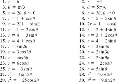
EXAMPLE 1 A Circle Centered at the Origin

Graph r = 3.

Solution Since θ is not specified, the point (3, θ) lies on the graph of r = 3 for any value of θ and is 3 units from the origin. We see in FIGURE 8.2.1 that the graph is the circle of radius 3 centered at the origin.

Alternatively, we know from (2) of Section 8.1 that r = ± so that r = 3 yields the familiar rectangular equation x² + y² = 3² of a circle of radius 3 centered at the origin.

FIGURE 8.2.1 Circle in Example 1

Circles Centered at the Origin In general, if a is any nonzero constant, the polar graph of

is a circle of radius |a| with center at the origin.

EXAMPLE 2 A Ray Through the Origin

Graph θ = π/4.

Solution Since r is not specified, the point (r, π/4) lies on the graph for any value of r. If r > 0, then this point lies on the half-line in the first quadrant; if r < 0, then the point lies on the half-line in the third quadrant. For r = 0, the point (0, π/4) is the pole or origin. Therefore, the polar graph of θ = π/4 is the line through the origin that makes an angle of π/4 with the polar axis or positive x-axis. See FIGURE 8.2.2.

FIGURE 8.2.2 Line in Example 2

Lines Through the Origin In general, if a is any nonzero real constant, the polar graph of

is a line through the origin that makes an angle of α radians with the polar axis.

EXAMPLE 3 A Spiral

Graph r = θ.

Solution As θ ≥ 0 increases, r increases and the points (r, θ) wind around the pole in a counterclockwise manner. This is illustrated by the blue portion of the graph in FIGURE 8.2.3. The red portion of the graph is obtained by plotting points for θ < 0.

FIGURE 8.2.3 Graph of equation in Example 3

Spirals Many graphs in polar coordinates are given special names. The graph in Example 3 is a special case of

where a is a constant. A graph of this equation is called a spiral of Archimedes. You are asked to graph other types of spiral curves in Problems 31 and 32 in Exercises 8.2.

In addition to basic point plotting, symmetry can often be utilized to graph a polar equation.

Symmetries of a snowflake

Symmetry As shown in FIGURE 8.2.4, a polar graph can have three types of symmetry. A polar graph is symmetric with respect to the y-axis if whenever (r, θ) is a point on the graph, (r, π – θ)is also a point on the graph. A polar graph is symmetric with respect to the x-axis if whenever (r, θ) is a point on the graph, (r, –θ) is also a point on the graph. Finally, a polar graph is symmetric with respect to the origin if whenever (r, θ) is on the graph, (–r, θ) is also a point on the graph.

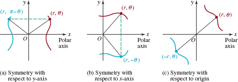
FIGURE 8.2.4 Symmetries of a polar graph

We have the following tests for symmetries in polar coordinates.

Because the polar description of a point is not unique, the graph of a polar equation may still have a particular type of symmetry even though the test for it may fail. For example, if replacing (r, θ) by (r, –θ) fails to give the original polar equation, the graph of that equation may still possess symmetry with respect to the x-axis. Therefore, if one of the replacement tests in (i)–(iii) of Theorem 8.2.1 fails to give the same polar equation, the best we can say is “no conclusion.”

In rectangular coordinates the description of a point is unique. Hence, in rectangular coordinates if a test for a particular type of symmetry fails, then we can definitely say that the graph does not possess that symmetry.

EXAMPLE 4 Graphing a Polar Equation

Graph r = 1 – cosθ.

Solution One way of graphing this equation is to plot a few well-chosen points corresponding to 0 ≤ θ ≤ 2π. As the following table shows

as θ advances from θ = 0 to θ = π/2, r increases from r = 0 (the origin) to r = 1. See FIGURE 8.2.5(a). As θ advances from θ = π/2 to θ = π, r continues to increase from r = 1 to its maximum value of r = 2. See FIGURE 8.2.5(b). Then, for θ = π to θ = 3π/2, r begins to decrease from r = 2 to r = 1. For θ = 3π/2 to θ = 2π, r continues to decrease and we end up again at the origin r = 0. See Figures 8.2.5(c) and 8.2.5(d).

By taking advantage of symmetry we could have simply plotted points for 0 ≤ θ ≤ π. From the trigonometric identity for the cosine function cos(–θ) = cosθ it follows from (ii) of Theorem 8.2.1 that the graph of r = 1 – cosθ is symmetric with respect to the x-axis. We can obtain the complete graph of r = 1 – cosθ by reflecting in the x-axis that portion of the graph given in FIGURE 8.2.5(b).

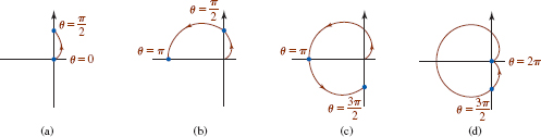
FIGURE 8.2.5 Graph of equation in Example 4

Cardioids The polar equation in Example 4 is a member of a family of equations that all have a “heart-shaped” graph that passes through the origin. A graph of any polar equation of the form

is called a cardioid. The only difference in the graph of these four equations is their symmetry with respect to the y-axis (r = a ± asinθ) or symmetry with respect to the x-axis (r = a ± acosθ). See FIGURE 8.2.6.

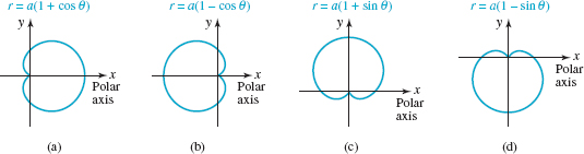
FIGURE 8.2.6 Cardioids

By knowing the basic shape and orientation of a cardioid, you can obtain a quick and accurate graph by plotting the four points corresponding to θ = 0, θ = π/2, θ = π, and θ = 3π/2.

Limaçons Cardioids are special cases of polar curves known as limaçons:

The shape of a limaçon depends on the relative magnitudes of a and b. Let us assume that a > 0 and b > 0. For a/b < 1, we get a limaçon with an interior loop as shown in FIGURE 8.2.7(a). When a = b or equivalently a/b = 1 we get a cardioid. For 1 < a/b < 2, we get a dimpled limaçon as shown in FIGURE 8.2.7(b). For a/b ≥ 2, the curve is called a convex limaçon. See FIGURE 8.2.7(c).

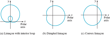
FIGURE 8.2.7 Three kinds of limaçons

EXAMPLE 5 A limaçon

The graph of r = 3 – sinθ is a convex limaçon, since a = 3, b = 1, and a/b = 3 > 2.

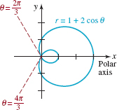
FIGURE 8.2.8 Graph of equation in Example 6

EXAMPLE 6 A limaçon

The graph of r = 1 + 2cosθ is a limaçon with an interior loop, since a = 1, b = 2, and a/b = < 1. For θ ≥ 0, notice in FIGURE 8.2.8 the limaçon starts at θ = 0 or (3, 0). The graph passes through the y-axis at (1, π/2) and then enters the origin (r = 0) for the first angle for which r = 0 or 1 + 2cosθ = 0 or cosθ = –. This implies that θ = 2π/3. At θ = π, the curve passes through (–1, π). The remainder of the graph can then be completed using the fact that it is symmetric with respect to the x-axis.

EXAMPLE 7 A Rose Curve

Graph r = 2cos2θ.

Solution Since

cos(–2θ) = cos2θ   and    cos2(π –θ) = cos2θ

we conclude by (i) and (ii) of the tests for symmetry that the graph is symmetric with respect to both the x- and the y-axes. A moment of reflection should convince you that we need only consider 0 ≤ θ ≤ π/2. Using the data in the following table, we see that

the dashed portion of the graph given in FIGURE 8.2.9 is that completed by symmetry. The graph is called a rose curve with four petals.

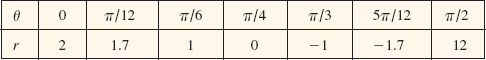
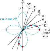
FIGURE 8.2.9 Graph of equation in Example 7

Rose Curves In general, if n is a positive integer, the graphs of

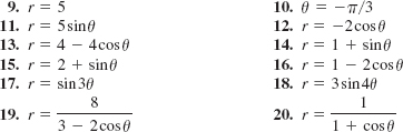
are called rose curves, although as you can see in FIGURE 8.2.10 the curve looks more like a daisy. When n is odd, the number of loops or petals of the curve is n; if n is even, the curve has 2n petals. To graph a rose curve we can start by graphing one petal. To begin, we find an angle θ for which r is a maximum. This gives the center line of the petal. We then find corresponding values of θ for which the rose curve enters the origin (r = 0). To complete the graph we use the fact that the center lines of the petals are spaced 2π/n radians (360/n degrees) apart if n is odd, and 2π/2n = π/n radians (180/n degrees) apart if n is even. In FIGURE 8.2.10 we have drawn the graph of r = asin5θ, a > 0. The spacing between the center lines of the five petals is 2π/5 radians (72°).

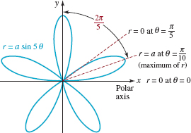
FIGURE 8.2.10 Rose curve with five petals

In Example 5 in Section 8.1 we saw that the polar equation r = 8cosθ is equivalent to the rectangular equation x² + y² = 8x. By completing the square in x in the rectangular equation, we recognize

(x – 4)² + y² = 16

as a circle of radius 4 centered at (4, 0) on the x-axis. Polar equations such as r = 8cosθ or r = 8sinθ are circles and are also special cases of rose curves. See FIGURE 8.2.11.

FIGURE 8.2.11 Graph of polar equation r = 8cosθ

Circles with Centers on an Axis When n = 1 in (6) we get

which are polar equations of circles passing through the origin with diameter |a| with centers (a/2, 0) on the x-axis (r = acosθ), or with centers (0, a/2) on the y-axis (r = asinθ). FIGURE 8.2.12 illustrates the graphs of the equations in (7) in the cases when a > 0 and a < 0.

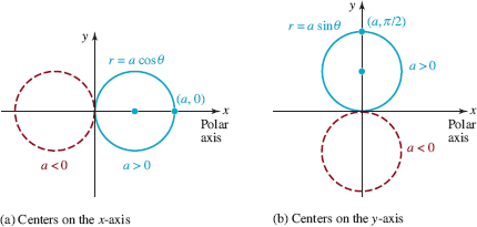
FIGURE 8.2.12 Circles through the origin with centers on an axis

Lemniscates If n is a positive integer, the graphs of

where a > 0, are called lemniscates. By (iii) of the tests for symmetry you can see the graphs of both of the equations in (8) are symmetric with respect to the origin. Moreover, by (ii) of the tests for symmetry the graph of r² = acos2θ is symmetric with respect to the x-axis. FIGURES 8.2.13(a) and 8.2.13(b) show typical graphs of the equations r² = acos2θ and r² = asin2θ, respectively.

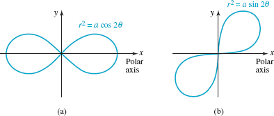
FIGURE 8.2.13 Lemniscates

Points of Intersection In rectangular coordinates we can find the points (x, y) where the graphs of two functions y = f(x) and y = g(x) intersect by equating the y-values. The real solutions of the equation f(x) = g(x) correspond to all the x-coordinates of the points where the graphs intersect. In contrast, problems may arise in polar coordinates when we try the same method to determine where the graphs of two polar equations r = f(θ) and r = g(θ) intersect.

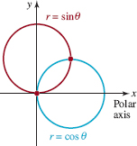
FIGURE 8.2.14 Intersecting circles in Example 8

EXAMPLE 8 Intersecting Circles

FIGURE 8.2.14 shows that the circles r = sinθ and r = cosθ have two points of intersection. By equating the r values, the equation sinθ = cosθ leads to θ = π/4. Substituting this value into either equation yields r = /2. Thus we have found only a single polar point (/2, π/4) where the graphs intersect. From the figure, it is apparent that the graphs also intersect at the origin. But the problem here is that the origin or pole is (0, π/2) on the graph of r = cosθ but is (0, 0) on the graph of r = sinθ. This situation is analogous to the curves reaching the same point at different times.

Rotation of Polar Graphs In Section 1.6 we saw that if y = f(x) is the rectangular equation of a function, then the graphs of y = f(x – c) and y = f(x + c), c > 0, are obtained by shifting the graph of f horizontally c units to the right and to the left, respectively. In contrast, if r = f(θ) is a polar equation, then the graphs of f(θ — γ) and f(θ + γ), where γ > 0, can be obtained by rotating the graph of f by an amount γ. Specifically:

• The graph of r = f(θ — γ) is the graph of r = f(θ) rotated counterclockwise about the origin by an amount γ.

• The graph of r = f(θ + γ) is the graph of r = f(θ) rotated clockwise about the origin by an amount γ.

For example, the graph of the cardioid r = a(1 + cosθ) is shown in FIGURE 8.2.6(a). The graph of r = a(1 + cos(θ — π/2)) is the graph of r = a(1 + cosθ) rotated counterclockwise about the origin by an amount π/2. Its graph then must be that given in FIGURE 8.2.6(c). This makes sense, because the difference formula of the cosine gives

r = a[1 + cosθ — π/2)] = a[1 + cosθ cos(π/2) + sinθ sin(π/2)] = a(1 + sinθ).

See the identity in (5) of Section 3.4.

Similarly, rotating r = a(1 + cosθ) counterclockwise about the origin by an amount π gives the equation

r = a[1 + cosθ — π)] = a[1 + cosθ cos π + sinθsinπ] = a(1 — cosθ)

whose graph is given in FIGURE 8.2.6(b). As another example, take a look again at FIGURE 8.2.13. From

we see that the graph of the lemniscate in FIGURE 8.2.13(b) is the graph in FIGURE 8.2.13(a) rotated counterclockwise about the origin by an amount π/4.

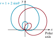
FIGURE 8.2.15 Graphs of polar equations in Example 9

EXAMPLE 9 Rotated Polar Graphs

Graph r = 1 + 2sinθ + π/4).

Solution The graph of the given equation is the graph of the limaçon r = 1 + 2sinθ rotated clockwise about the origin by an amount π/4. In FIGURE 8.2.15 the blue graph is that of r = 1 + 2sinθ and the red graph is the rotated graph.

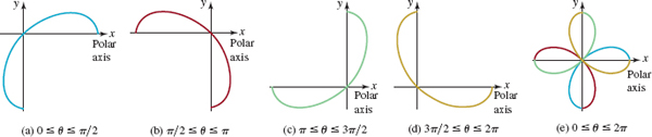
FIGURE 8.2.16 Plotting r = 2cos2θ

8.2Exercises Answers to selected odd-numbered problems begin on page ANS-21.

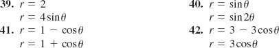
In Problems 1-30, identify by name the graph of the given polar equation. Then sketch the graph of the equation.

In Problems 31 and 32, the graph of the given equation is a spiral. Sketch its graph.

31. r = 2^θ, θ ≥ 0(logarithmic)

32. rθ = π, θ > 0(hyperbolic)

In Problems 33-38, find an equation of the given polar graph.

FIGURE 8.2.17 Graph for Problem 33

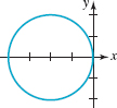
FIGURE 8.2.18 Graph for Problem 34

FIGURE 8.2.19 Graph for Problem 35

FIGURE 8.2.20 Graph for Problem 36

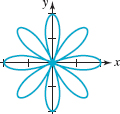
FIGURE 8.2.21 Graph for Problem 37

FIGURE 8.2.22 Graph for Problem 38

In Problems 39-42, find the points of intersection of the graphs of the given pair of polar equations.

Calculator/CAS Problems

43. Use a graphing utility to obtain the graph of the bifolium r = 4sinθcos²θ and the circle r = sinθ on the same axes. Find all points of intersection of the graphs.

44. Use a graphing utility to verify that the cardioid r = 1 + cosθ and the lemniscate r² = 4cosθ intersect at four points. Find these points of intersection of the graphs.

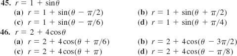
In Problems 45 and 46, the graphs of the equations (a)-(d) represent a rotation of the graph of the given equation. Try sketching these graphs by hand. If you have difficulties, then use a calculator or CAS.

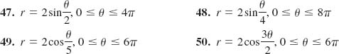
In Problems 47-50, use (9) to parameterize the curve whose polar equation is given. Use a graphing utility to obtain the graph of the resulting set of parametric equations.

For Discussion

In Problems 51 and 52, suppose r = f(θ) is a polar equation. Graphically interpret the given property.

51. f(–θ) = f(θ)(even function)

52. f(–θ) = –f(θ)(odd function)

8.3 Conic Sections in Polar Coordinates

Introduction In Chapter 7 we derived equations for the parabola, ellipse, and hyperbola using the distance formula in rectangular coordinates. By using polar coordinates and the concept of eccentricity, we can now give one general definition of a conic section that encompasses all three curves. Conic Sections in Polar Coordinates

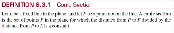
The fixed line L is called a directrix, and the point F is a focus. The fixed constant is the eccentricity e of the conic. As FIGURE 8.3.1 shows, the point P lies on the conic if and only if

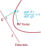
FIGURE 8.3.1 Geometric interpretation of (1)

where Q denotes the foot of the perpendicular from P to L. In (1), if

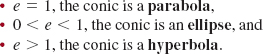
FIGURE 8.3.2 Polar coordinate interpretation of (1)

Polar Equations of Conics Equation (1) is readily interpreted using polar coordinates. Suppose F is placed at the pole and L is p units (p > 0) to the left of F perpendicular to the extended polar axis. We see from FIGURE 8.3.2 that (1) written as d(P, F) = ed(P, Q) is the same as

Solving for r yields

To see that (3) yields the familiar equations of the conics, let us superimpose a rectangular coordinate system on the polar coordinate system with origin at the pole and the positive x-axis coinciding with the polar axis. We then express the first equation in (2) in rectangularcoordinates and simplify:

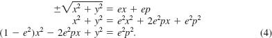
Choosing e = 1, (4) becomes

The last equation is the standard form of a parabola whose axis is the x-axis, vertex is at and, consistent with the placement of F, whose focus is at the origin.

It is a good exercise in algebra to show that (3) yields standard form equations of an ellipse in the case 0 < e < 1 and a hyperbola in the case e > 1. See Problem 43 in Exercises 8.3. Thus, depending on the value of e, the polar equation (3) can have three possible graphs as shown in FIGURE 8.3.3.

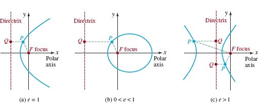
FIGURE 8.3.3 Graphs of equation (3)

If we had placed the focus F to the left of the directrix in our derivation of the polar equation (3), then the equation r = ep/(1 + ecosθ) would be obtained. When the directrix L is chosen parallel to the polar axis (that is, horizontal), then the equation of the conic is found to be either r = ep/(1 — esinθ)or r = ep/(1 + esinθ). A summary of the preceding discussion is given next.

is a conic section with focus at the origin and axis along a coordinate axis. The axis of the conic section is along the x-axis for equations of the form (5) and along the y-axis for equations of the form (6). The conic is a parabola if e = 1, an ellipse if 0 < e < 1, and a hyperbola if e > 1.

EXAMPLE 1Identifying Conics

Identify each of the following conics

Solution (a) A term-by-term comparison of the given equation with the polar form r = ep/(1 – esinθ) enables us to make the identification e = 2. Hence the conic is a hyperbola.

(b) In order to identify the conic section, we divide the numerator and the denominator of the given equation by 4. This puts the equation into the form

Then by comparison with r = ep/(1 + ecosθ) we see that Hence the conic is an ellipse.

Graphs A rough graph of a conic defined by (5) or (6) can be obtained by knowing the orientation of its axis, finding the x-and y-intercepts, and finding the vertices. In the case of (5),

 

• the two vertices of the ellipse or a hyperbola occur at θ = 0 and θ = π; the vertex of a parabola can occur at only one of the values: θ = 0 or θ = π.

For (6),

• the two vertices of an ellipse or a hyperbola occur at θ = π/2 and θ = 3π/2; the vertex of a parabola can occur at only one of the values θ = π/2 or θ = 3π/2.

 

EXAMPLE 2Graphing a Conic

Solution By writing the equation as we see that the eccentricity is and so the conic is an ellipse. Moreover, because the equation is of the form given in (6), we know that the axis of the ellipse is vertical along the y-axis. Now in view of the discussion preceding this example, we obtain:

The graph of the equation is given in FIGURE 8.3.4.

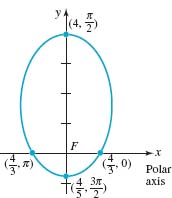
FIGURE 8.3.4 Graph of polar equation in Example 2

EXAMPLE 3Graphing a Conic

Solution Inspection of the equation shows that it is of the form given in (5) with e = 1. Hence the conic section is a parabola whose axis is horizontal along the x-axis. Since r is undefined at θ = 0, the vertex of the parabola occurs at θ = π:

The graph of the equation is given in figure 8.3.5.

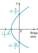
FIGURE 8.3.5 Graph of polar equation in Example 3

EXAMPLE 4Graphing a Conic

Solution From (5) we see that e = 2 and so the conic section is a hyperbola whose axis is horizontal along the x-axis. The vertices, the endpoints of the transverse axis of the hyperbola, occur at θ = 0 and at θ = π:

The graph of the equation is given in FIGURE 8.3.6.

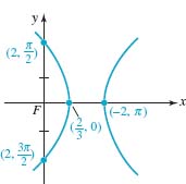
FIGURE 8.3.6 Graph of polar equation in Example 4

Rotated Conics We saw in Section 8.2 that graphs of r = f(θ — γ) and r = f (θ + γ), γ > 0, are rotations of the graph of the polar equation r = f (θ) about the origin by an amount γ. Thus

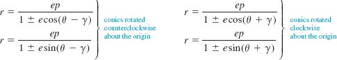
EXAMPLE 5Rotated Conic

In Example 2 we saw that the graph of is an ellipse with major axis along the y-axis. This is the blue graph in FIGURE 8.3.7 The graph of r = is the red graph in FIGURE 8.3.7 and is a counterclockwise rotation of the blue graph by the amount 2π/3 radians (or) about the origin. The major axis of the red graph lies along the line θ = 7 π/6

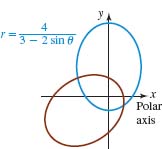
FIGURE 8.3.7 Graphs of polar equations in Example 5

Applications Equations of the type in (5) and (6) are well suited to describe a closed orbit of satellite around the Sun (Earth or Moon) since such an orbit is an ellipse with the Sun (Earth or Moon) at one focus. Suppose that an equation of the orbit is given by r = ep/(1 — ecosθ), 0 < e < 1, and r_p is the value of r at perihelion (perigee or perilune) and r_a is the value of r at aphelion (apogee or apolune). These are the points in the orbit, occurring on the x-axis, at which the satellite is closest and farthest, respectively, from the Sun (Earth or Moon). See FIGURE 8.3.8. It is left as an exercise to show that the eccentricity e of the orbit is related to r_p and r_a by

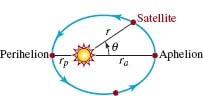
FIGURE 8.3.8 Orbit of satellite

EXAMPLE 6Polar Equation of an Orbit

Find a polar equation of the orbit of the planet Mercury around the Sun if r_p = 2.85 × 10⁷ miles and r_a = 4.36 × 10⁷ miles.

Solution From (7), the eccentricity of Mercury–s orbit is

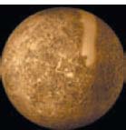
Mercury is the closest planet to the Sun

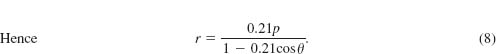
All we need to do now is to solve for the quantity 0.21p. To do this we use the fact that aphelion occurs at θ = 0:

The last equation yields 0.21p = 3.44 × 10⁷. Substituting this value of 0.21p in (8) yields the polar equation

of Mercury–s orbit.

 

8.3Exercises Answers to selected odd-numbered problems begin on page ANS-22.

In Problems 1-10, determine the eccentricity, identify the conic, and sketch its graph.

1.

2.

3.

4.

5.

6.

7.

8.

9.

10.

In Problems 11-14, determine the eccentricity e of the given conic. Then convert the polar equation to a rectangular equation and verify that e = c/a.

11.

12.

13.

14.

In Problems 15-20, find a polar equation of the conic with focus at the origin that satisfies the given conditions.

15. e = 1, directrix x = 3

16. e = , directrix y = 2

17. e = , directrix y = – 2

18. e = , directrix x = 4

19. e = 2, directrix x = 6

20. e = 1, directrix y = –2

21.Find a polar equation of the conic in Problem 15 if the graph is rotated clockwise about the origin by an amount 2π/3.

22.Find a polar equation of the conic in Problem 16 if the graph is rotated counterclockwise about the origin by an amount π/6.

In Problems 23-28, find a polar equation of the parabola with focus at the origin and the given vertex.

23.

24. (2, π)

25.

26. (2, 0)

27.

28.

In Problems 29-32, find the polar coordinates of the vertex or vertices of the given rotated conic.

29.

30.

31.

32.

Miscellaneous Applications

33.Perigee Distance A communications satellite is 12,000 km above the Earth at its apogee. The eccentricity of its elliptical orbit is 0.2. Use (7) to find its perigee distance.

34.Orbit Find a polar equation r = ep/(1 – ecosθ) of the orbit of the satellite in Problem 33.

35.Earth–s Orbit Find a polar equation of the orbit of the Earth around the Sun if r_p = 1.47 × 10⁸ km and r_a = 1.52 × 10⁸km.

36.Comet Halley (a) The eccentricity of the elliptical orbit of Comet Halley is 0.97 and the length of the major axis of its orbit is 3.34 × 10⁹ mi. Find a polar equation of its orbit of the form r = ep/(1 – ecosθ).

(b) Use the equation in part (a) to obtain r_p and r_a for the orbit of Comet Halley.

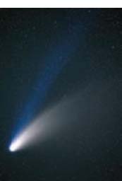
Next visit of Comet Halley to the Solar System will be in 2061

Calculator/CAS Problems

The orbital characteristics (eccentricity, perigee, and major axis) of a satellite near the Earth gradually degrade over time due to many small forces acting on the satellite other than the gravitational force of the Earth. These forces include atmospheric drag, gravitational attractions of the Sun and the Moon, and magnetic forces. Approximately once a month tiny rockets are activated for a few seconds in order to “boost” the orbital characteristics back into the desired range. Rockets are turned on longer to a major change in the orbit of a satellite. The most fuel efficient way to move from an inner orbit to an outer orbit, called a Hohmann transfer, is to add velocity in the direction of flight at the time the satellite reaches perigee on the inner orbit, follow the Hohmann transfer ellipse halfway around to its apogee, and add velocity again to achieve the outer orbit. A similar process (subtracting velocity at apogee on the outer orbit and subtracting velocity at perigee on the Hohmann transfer orbit) moves a satellite from an outer orbit to an inner orbit.

In Problems 37-40, use a graphing calculator or CAS to superimpose the graphs of the given three polar equations on the same coordinate axes. Print out your result and use a colored pencil to trace out the Hohmann transfer.

37. Inner orbit Hohmann transfer outer orbit

38. Inner orbit Hohmann transfer outer orbit

39. Inner orbit r = 9, Hohmann transfer outer orbit r = 51

40. Inner orbit Hohmann transfer outer orbit

In Problems 41 and 42, use a calculator or CAS to superimpose the graphs of the given two polar equations on the same coordinate axes.

41.

42.

For Discussion

43. Show that (3) yields standard form equations of an ellipse in the case 0 < e < 1 and a hyperbola in the case e < 1.

44. Use the equation r = ed/(1 – ecosθ) to derive the result in (7).

CHAPTER 8Review Exercises Answers to selected odd-numbered problems begin on page ANS-22.

A. True/False__________________________________________________

In Problems 1-12, answer true or false.

1. Rectangular coordinates of a point in the plane are unique.____

2. The graph of the polar equation r = 5 secθ is a line.____

3. (3, π/6) and (–3, –5π/6) are polar coordinates of the same point.____

4. The graph of the ellipse is nearly circular.____

5. The graph of the rose curve r = 5 sin6θ has six petals.____

6. The graph of r = 2 + 4 sinθ is a limaçon with an interior loop.____

7. The graph of the polar r² = 4 sin2θ is symmetric with respect to the origin.____

8. The graphs of the cardioids r = 3 + 3 cosθ and r = –3 + 3 cosθ are the same.____

9. The point (4, 3π/2) is not on the graph of r = 4 cos 2θ, because its coordinates do not satisfy the equation.____

10. The graph of a limaçon without an interior loop does not pass through the origin.____

11. The terminal side of the angle θ is always in the same quadrant as the point (r, θ).____

12. The eccentricity e of a parabola satisfies 0 < e < 1.____

B. Fill in the Blanks______________________________________________

In Problems 1-12, fill in the blanks.

1. The rectangular coordinates of the point with polar coordinates ___________.

2. Approximate polar coordinates of the point with rectangular coordinates (–1, 3) are___________.

3. Polar coordinates of the point with rectangular coordinates (0, –10) are___________.

4. On the graph of the polar equation r = 4 cosθ, two pairs of coordinates of the pole or origin are___________.

5. The radius of the circle r = cos θ is___________.

6. If a > 0, the center of the circle r = –2asinθ is___________.

7. The conic section is a___________.

8. In polar coordinates, the graph of θ = π/3 is a___________.

9. The name of the polar graph of r = 2 + sinθ is___________.

10. center___________, foci___________, vertices___________

11. Using one word, the graph of the polar equation r = 3^θ is a___________.

12. The point with polar coordinates (4, π) is a(n)____-intercept of the graph of

C. Review Exercises_______________________________________________

In Problems 1 and 2, find a rectangular equation that has the same graph as the given polar equation.

1. r = cos θ 1 sinθ

2. r(cosθ + sinθ) = 1

In Problems 3 and 4, find a polar equation that has the same graph as the given rectangular equation.

3. x² + y² – 4y = 0

4. (x² + y² – 2x)² = 9(x² + y²)

5. Determine the rectangular coordinates of the vertices of the ellipse whose polar equation is r = 2/(2 – sinθ).

6. Find a polar equation of the hyperbola with focus at the origin, vertices (in rectangular coordinates) and eccentricity 2.

In Problems 7 and 8, find polar coordinates satisfying (a) r > 0, –π < θ ≤ π, and (b) r < 0, –π < θ ≤ π, for each point given in rectangular coordinates.

7.

8.

In Problems 15-26, identify and sketch the graph of the given polar equation.

In Problems 21 and 22, give an equation of the given polar graph.

FIGURE 8.R.1 Graph for Problem 21

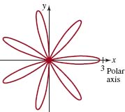
FIGURE 8.R.2 Graph for Problem 22

In Problems 23 and 24, the graph of the given polar equation is rotated about the origin by the indicated amount. (a) Find a polar equation of the new graph. (b) Find a rectangular equation for the new graph.

23. r = 2 cosθ; counterclockwise, π/4

24. r = 1/(1 + cos θ); clockwise, π/6

25. (a) Show that the graph of the polar equation

   r = a sinθ + b cos θ

   for a ≠ 0 and b ≠ 0, is a circle.

 (b) Determine the center and radius of the circle in part (a).

26. (a) Find a rectangular equation that has the same graph as the given polar equation: rcos θ = 1, rcos(θ – π/3) = 1, r = 1. Sketch the graph of each equation.

(b) How are the graphs of rcos θ = 1 and rcos(θ — π/3) = 1 related?

(c) Show that rectangular point is on the graphs of rcos(θ – π/3) = 1 and r = 1.

(d) Use the information in parts (a) and (c) to explain how the graphs of rcos(θ – π/3) = 1 and r = 1 are related.

In Problems 27 and 28, (a) use a graphing utility to obtain the graph of the given polar equation. (b) Find a rectangular that has the same graph as the polar equation

27. r = sinθ tanθ, – π/2 < θ < π/2, (cissoid)

28. r = 2 + sec θ, 0 < θ < π, (conchoid)