1 Prerequisites for Trigonometry

In This Chapter

1.1 The Real Number Line

1.2 The Rectangular Coordinate System

1.3 Circles and Graphs

1.4 Equations of Lines

1.5 Functions and Graphs

1.6 Symmetry and Transformations

1.7 Linear and Quadratic Functions

1.8 Combining Functions

1.9 Inverse Functions

1.10 Building a Function from Words

      Chapter 1 Review Exercises

The correspondence between the students in a class and the set of desks filled by these students is an example of a function.

A Bit of History If the question “What is the most important mathematical concept?” were posed to a group of mathematicians, mathematics teachers, and scientists, certainly the term function would appear near or even at the top of the list of their responses. In this opening chapter, we will focus primarily on the definition and the graphical interpretation of a function.

The word “function” was probably introduced by the German mathematician and “co-inventor” of calculus, Gottfried Wilhelm Leibniz (1646-1716), in the late seventeenth century and stems from the Latin word “functo,” meaning to act or perform. In the seventeenth and eighteenth centuries mathematicians had only the most intuitive notion of a function. To many of them, a functional relationship between two variables was given by some smooth curve or by an equation involving the two variables. Although formulas and equations play an important role in the study of functions, we will see in Section 1.5 that the “modern” interpretation of a function (dating from the middle of the nineteenth century) is that of a special type of correspondence between the elements of two sets.

In Chapter 3 we examine the properties and graphs of the trigonometric functions.

1.1 The Real Number Line

Introduction For any two distinct real numbers a and b, there is always a third real number between them; for example, their average (a + b)/2 is midway between them. Similarly, for any two distinct points A and B on a straight line, there is always a third point between them; for example, the midpoint M of the line segment AB. There are many such similarities between the set R of real numbers and the set of points on a straight line that suggest using a line to “picture” the set of real numbers R = R⁻ ∪ {0} ∪ R⁺. This can be done as follows.

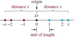
FIGURE 1.1.1 Number line

Real Number Line Given any straight line, we choose a point O on the line to represent the number 0. This particular point is called the origin. If we now select a line segment of unit length as shown in FIGURE 1.1.1, each positive real number x can be represented by the point at a distance x to the right of the origin. Similarly, each negative real number –x can be represented by the point at a distance x to the left of the origin. This association results in a one-to-one correspondence between the set R of real numbers and the set of points on a straight line, called the real number line. For any given point P on the number line, the number p, which corresponds to this point, is called the coordinate of P. Thus the set R ^— of negative real numbers consists of the coordinates of points to the left of the origin, the set R ⁺ of negative real numbers consists of the coordinates of points to the right of the origin; the number 0 is the coordinate of the origin O. See FIGURE 1.1.2.

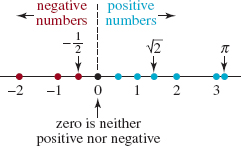
FIGURE 1.1.2 Positive and negative directions on the number line

In general, we will not distinguish between a point on the number line and its coordinate. Thus, for example, we will sometimes refer to the point on the real number line with coordinate 5 as “the point 5.”

Less Than and Greater Than Two real numbers a and b, a ≠ b, can be compared by the order relation less than. We have the following definition.

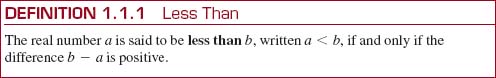
If a is less than b, then equivalently we can say that b is greater than a and write b < a. For example, −7 < 5, because 5 − (− 7) = 12 is positive. Alternatively, we can write 5 > − 7.

FIGURE 1.1.3 The number a is to the Left of the number b

EXAMPLE 1 An Inequality

Using the order relation greater than, compare the real numbers π and 22/7.

Solution From π = 3.1415…and 22/7 = 3.1428…, we find that

Since this difference is positive, we conclude that 22/7 > π

Inequalities The number line is useful in demonstrating order relations between two real numbers a and b. As shown in FIGURE 1.1.3, we say that the number a is less than the number b, and write a < b, whenever the number a lies to the left of the number b on the number line. Equivalently, because the number b lies to the right of a on the number line we say that b is greater than a and write b > a. For example, 4 < 9 is the same as 9 > 4. We also use the notation a≤b if the number a is less than or equal to the number b. Similarly, b≥a means b is greater than or equal to a. For example, 2 ≤ 5 since 2 < 5. Also, 4 ≥ 4 because 4 = 4.

For any two real numbers a and b, exactly one of the following is true:

The property given in (1) is called the trichotomy law.

Terminology The symbols <, >, ≤, and ≥ are called inequality symbols and expressions such as a < b or b ≥ a are called inequalities. An inequality a < b is often called a strict inequality, whereas an inequality such as b ≥ a is called a non-strict inequality. The inequality a > 0 means the number a lies to the right of the number 0 on the number line and so a is positive. We signify that a number a is negative by the inequality a < 0. Because the inequality a ≤ 0 means a is either greater than 0 (positive) or equal to 0 (which is neither positive nor negative), we say that a is nonnegative. Similarly, if a ≥ 0, we say that a is nonpositive.

Inequalities also have the following transitivity property.

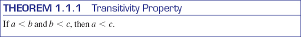
For example, if x < 12 and 12 < y, we conclude from the transitivity property that x < y. Theorem 1.2.1 can easily be visualized on the number line by placing a anywhere on the line, b to the right of a, and the number c to the right of b.

Absolute Value We can also use the real number line to picture distance. As shown in FIGURE 1.1.4, the distance from the point 3 to the origin is 3 units, and the distance from the point – 3 to the origin is 3, or – (–3), units. It follows from our discussion of the number line that, in general, the distance from any number to the origin is the “unsigned value” of that number.

More precisely, as shown in FIGURE 1.1.5, for any positive real number x, the distance from the point x to the origin is x, but for any negative number y, the distance from the point y to the origin is –y. Of course, for x = 0, the distance to the origin is 0. The concept of the distance from a point on the number line to the origin is described by the notion of the absolute value of a real number.

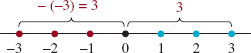
FIGURE 1.1.4 Distance on the number line

FIGURE 1.1.5 The distance from 0 to x is x the distance from 0 to y is −y

EXAMPLE 2 Absolute Values

Since 3 and √2 are positive numbers,

|3| = 3 and | √2| = √2.

But since −3and −√2are negative numbers; that is, −3 < 0 and −√2 <0, we see

|−3| = −(−3) = 3 and |−√2| = − (−√2) = √2.

EXAMPLE 3 Absolute Values

(a)|2 − 2 | = |0| = 0← from (2), 0 ≥ 0

(b)|2 − 6| = |−4| = − (−4) = 4 ← from (2), −4 < 0

(c)|2 | − |−5| = 2 − [−(−5)] = 2 − 5 = −3 ← from (2), −5 < 0

EXAMPLE 4 Absolute Value

Find | √2 − 31.

Solution To find | √22 − 31, we must determine first whether the number √22 − 3 is positive or negative. Since √22 √2 1.4, we see that √22 − 3 is a negative number. Thus,

Note of Caution

It is a common mistake to think that – y represents a negative number because the symbol y is preceded by a minus sign. We emphasize that if y represents a negative number, then the negative of y, that is, −y, is a positive number. Hence, if y is negative, then |y| = −y.

EXAMPLE 5 Value of an Absolute Value Expression

Find |x − 6| if (a) x > 6, (b) x = 6, and (c) x < 6.

Solution

(a) If x > 6, then x − 6 is positive. Then from the definition of absolute value in (2), we conclude that |x − 6| = |x − 6|.

(b) If x = 6, then x − 6 = 0;hence |x − 6| = |0| = 0.

(c) If x < 6, then x − 6 is negative and we have that |x − 6| = − (x − 6) = 6 − x.

See Appendix A for a review of equations and inequalities involving absolute values.

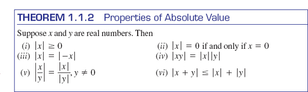
For any real number x and its negative, − x, the distance to the origin is the same. That is, x = − x. This is one of several special properties of the absolute value, which we list in the following theorem.

Restating these properties in words is one way of increasing your understanding of them. For example, property (i) states that the absolute value of a quantity is always nonnegative. Property (iv) says that the absolute value of a product equals the product of the absolute values of the two factors. Part (vi) of Theorem 1.2.2 is an important property and is called the triangle inequality.

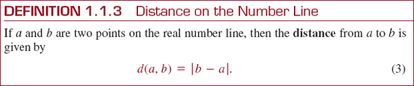
Distance Between Points The concept of absolute value not only describes the distance from a point to the origin. It is also useful in finding the distance between two points on the number line. Since we want to describe distance as a positive quantity, we subtract one coordinate from the other and then take the absolute value of the difference. See FIGURE 1.1.6.

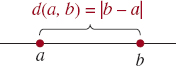
FIGURE 1.1.6 Distance on the number line

EXAMPLE 6 Distances

(a) The distance from −5 to 2 is

(b) The distance from 3 to √2 is

We see that the distance from a to b is the same as the distance from b to a, since by (iii) of Theorem 1.1.2,

Thus, d(a, b) = d(b, a).

Coordinate of the Midpoint Definition 1.1.3 can be used to find an expression for the midpoint of a line segment. The midpoint m of the line segment joining a and b is the average of the two endpoints:

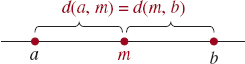
FIGURE 1.1.7 Distance from a to m equals the distance from m to b

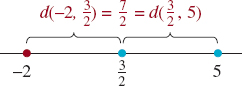
FIGURE 1.1.8 Midpoint in Example 7

EXAMPLE 7 Midpoint

From (4), the midpoint of the line segment joining the points 5 and −2 is

See FIGURE 1.1.8.

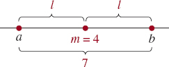
FIGURE 1.1.9 Distances are equal in Example 8

EXAMPLE 8 Given the Midpoint

The line segment joining a to b has midpoint m = 4. If the distance from a to b is 7, find a and b.

Solution As we can see in FIGURE 1.1.9, since m is the midpoint,

Thus, 2l = 7 or . We now have and

In Problems 1 and 2, construct a number line and locate the given points on it.

1.

2.

In Problems 3-10, write the statement as an inequality.

3. x is positive

4. y is nonnegative

5. x + y is nonnegative

6. a is less than −3

7. b is greater than or equal to 100

8. c − 1 is less than or equal to 5

9. |t−1| is less than 50

10. |s + 4| is greater than or equal to 7

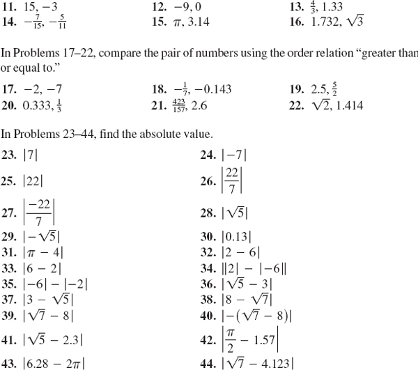
In Problems 11-16, compare the pair of numbers using the order relation “less than.”

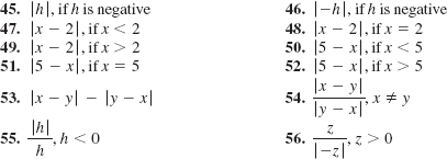
In Problems 45-56, write the expression without using absolute value symbols.

In Problems 57–64, (a) find the distance between the given points and (b) find the coordinate of the midpoint of the line segment joining the given points.

In Problems 65–72, m is the midpoint of the line segment joining a (the left endpoint) and b (the right endpoint). Use the given conditions to find the indicated values.

In Problems 73–80, determine which statement from the trichotomy law is true for the given pair of numbers a, b.

Miscellaneous Applications

81. How Far?Greg, Tricia, Ethan, and Natalie live on Real Street. Tricia lives a mile from Greg, and Ethan lives one-half mile from Tricia. Natalie lives halfway between Ethan and Tricia. How far does Natalie live from Greg? [Hint: There are two solutions.]

82. Shipping Distance A company that owned one manufacturing plant next to a river bought two additional manufacturing plants, one x miles upstream and the other y miles downstream. Now the company wants to build a processing plant located so that the total shipping distance from the processing plant should be built at the same location as the original manufacturing plant. [Hint: Think of the plants as being located at 0, x, and –y on a number line.] See FIGURE 1.1.10. Using absolute values, find an expression for the total shipping distance if the processing plant is located at point d.

FIGURE 1.1.10 Plants in Problem 82

For Discussion

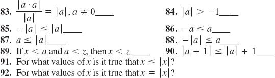
For Problems 83-90, answer true or false for any real number a.

93. Use Definition 1.1.2 to prove that | xy | = | x | y | for any real numbers x and y.

94. Use Definition 1.1 .2 to prove that | x/y | = | x | |/ y | for any real number x and any nonzero real number y.

95. Under what conditions does equality hold in the triangle inequality; that is, when is it true that |a + b| = |a| + |b|?

96. Use the triangle inequality to prove |a – b|≤|a| + |b|.

97. Use the triangle inequality to prove |a – b | ≤ | a | − | b |. [Hint: a = (a − b) + b.]

98. Prove the midpoint formula (4).

1.2 The Rectangular Coordinate System

Introduction In Section 1.1 we saw that each real number can be associated with exactly one point on the number, or coordinate, line. We now examine a correspondence between points in a plane and ordered pairs of real numbers.

The Coordinate Plane A rectangular coordinate system is formed by two perpendicular number lines that intersect at the point corresponding to the number 0 on each line. This point of intersection is called the origin and is denoted by the symbol O. The horizontal and vertical number lines are called the x-axis and the y-axis, respectively. These axes divide the plane into four regions, called quadrants, which are numbered as shown in FIGURE 1.2.1(a). As we can see in FIGURE 1.2.1(b), the scales on the x- and y-axes need not be the same. Throughout this text, if tick marks are not labeled on the coordinates axes, as in FIGURE 1.2.1(a), then you may assume that one tick corresponds to one unit. A plane containing a rectangular coordinate system is called an xy-plane, a coordinate plane, or simply 2-space.

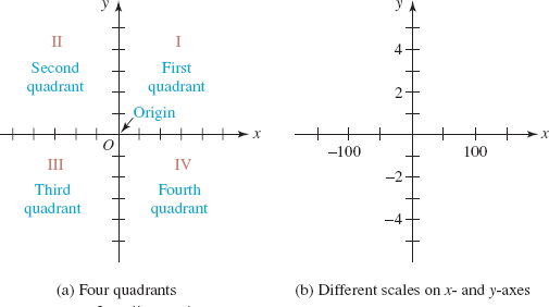
FIGURE 1.2.1 Coordinate plane

The rectangular coordinate system and the coordinate plane are also called the Cartesian coordinate system and the Cartesian plane after the famous French mathematician and philosopher Ren&Copy; Descartes (1596-1650).

Coordinates of a Point Let P represent a point in the coordinate plane. We associate an ordered pair of real numbers with P by drawing a vertical line from P to the x-axis and a horizontal line from P to the y-axis. If the vertical line intersects the x-axis at the number a and the horizontal line intersects the y-axis at the number b, we associate the ordered pair of real numbers (a, b) with the point. Conversely, to each ordered pair (a, b) of real numbers, there corresponds a point P in the plane. This point lies at the intersection of the vertical line through a on the x-axis and the horizontal line passing through b on the y-axis. Hereafter, we will refer to an ordered pair as a point and denote it by either P(a, b) or (a, b).^* The number a is the x-coordinate of the point and the number b is the y-coordinate of the point and we say that P has coordinates (a, b). For example, the coordinates of x the origin are (0, 0). See FIGURE 1.2.2.

The algebraic signs of the x-coordinate and the y-coordinate of any point (x, y) in each of the four quadrants are indicated in FIGURE 1.2.3. Points on either of the two axes are not considered to be in any quadrant. Since a point on the x-axis has the form (x, 0), an equation that describes the x-axis is y = 0. Similarly, a point on the y-axis has the form (0, y) and so an equation of the y-axis is x = 0. When we locate a point in the coordinate plane corresponding to an ordered pair of numbers and represent it using a solid dot, we say that we plot or graph the point.

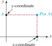
FIGURE 1.2.2 Point with coordinates (a, b)

FIGURE 1.2.3 Algebraic signs of coordinates in the four quadrants

EXAMPLE 1 Plotting Points

Plot the points A (1, 2), B(−4, 3), , D(0, 4), and E(3.5, 0). Specify the quadrant in which each point lies.

Solution The five points are plotted in the coordinate plane in FIGURE 1.2.4. Point A lies in the first quadrant (quadrant I), B in the second quadrant (quadrant II), and C is in the third quadrant (quadrant III). Points D and E, which lie on the y- and the x-axes, respectively, are not in any quadrant.

FIGURE 1.2.4 Five points in Example 1

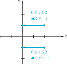
FIGURE 1.2.5 Set of points in Example 2

EXAMPLE 2 Plotting Points

Sketch the set of points (x, y) in the xy-plane that satisfy both 0≤x≤2 and |y| = 1.

Solution First, the absolute-value equation |y| = 1 implies that y = −l or y = 1.(See Appendix A.) Thus the points that satisfy the given conditions are the points whose coordinates (x, y) simultaneously satisfy the conditions: each x-coordinate is a number in the closed interval [0, 2] and each y-coordinate is either y = − 1 or y = 1.For example, (1, 1), and (2, −1) are a few of the points that satisfy the two conditions. Graphically, the set of all points satisfying the two conditions are points on the two parallel line segments shown in FIGURE 1.2.5.

EXAMPLE 3 Regions Defined by Inequalities

Sketch the set of points (x, y) in the xy-plane that satisfy each of the following conditions.

(a) xy < 0

(b) | y | ≥ 2

Solution (a) From the sign properties of products, we know that a product of two real numbers x and y is negative when one of the numbers is positive and the other is negative. Thus, xy < 0when x > 0and y < 0 or when x < 0and y > 0. We see from FIGURE 1.2.3 that xy < 0 for all points (x, y) in the second and fourth quadrants. Hence we can represent the set of points for which xy < 0 by the shaded regions in FIGURE 1.2.6. The coordinate axes are shown as dashed lines to indicate that the points on these axes are not included in the solution set.

(b) The inequality |y| ≥ 2 means that either y ≥ 2 or y≥−2. (See Appendix A.) Since x is not restricted in any way it can be any real number, and so the points (x, y) for which

can be represented by the two shaded regions in FIGURE 1.2.7. We use solid lines to represent the boundaries y = −2 and y = 2 of the region to indicate that the points on these boundaries are included in the solution set.

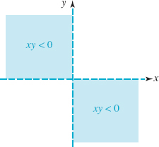
FIGURE 1.2.6 Region in the xy-plane satisfying condition in (a) of Example 3

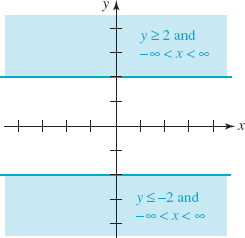
FIGURE 1.2.7 Region in the xy-plane satisfying condition in (b) of Example 3

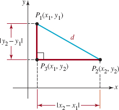
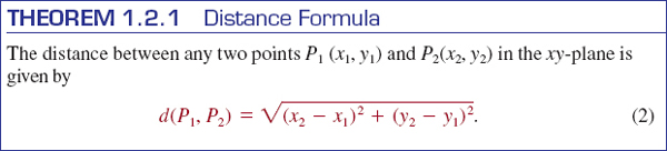
FIGURE 1.2.8 Distance between points P₁ and P₂

Distance Formula Suppose P(x₁, y₁) and P₂(x₂, y₂) are two distinct points in the xy-plane that are not on a vertical line or on a horizontal line. As a consequence, P₁, P₂, and P₃ (x₁, y₂) are vertices of a right triangle as shown in FIGURE 1.2.8. The length of the side P₃P₂is |x₂ – x₁|, and the length of the side _P1P3 is |y₂ – y₂. If we denote the length of P₁P₂ by d, then

by the Pythagorean theorem. Since the square of any real number is equal to the square of its absolute values, we can replace the absolute-value signs in (1) with parentheses. The distance formula given next follows immediately from (1).

Although we derived this equation for two points not on a vertical or horizontal line, (2) holds in these cases as well. Also, because (x₂ – x₁)² = (x₁ – x₂)², it makes no difference which point is used first in the distance formula, that is, d(P1, P2) = d(P2, P1).

EXAMPLE 4 Distance Between Two Points

Find the distance between the points A(8, -5) and B(3, 7).

Solution From (2) with A and B playing the parts of P₁ and P₂:

The distance d is illustrated in FIGURE 1.2.9.

EXAMPLE 5 Three Points Form a Triangle

Determine whether the points P₁(7, 1), P₂(−4, −1), and P₃(4, 5) are the vertices of a right triangle.

Solution From plane geometry we know that a triangle is a right triangle if and only if the sum of the squares of the lengths of two of its sides is equal to the square of the length of the remaining side. Now, from the distance formula (2), we have

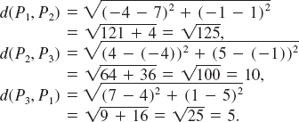
Since

we conclude that P₁, P₂, and P₃ are the vertices of a right triangle with the right angle at P₃. See FIGURE 1.2.10.

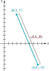
FIGURE 1.2.9 Distance between two points in Example 4

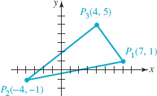
FIGURE 1.2.10 Triangle in Example 5

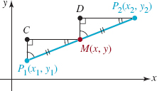
FIGURE 1.2.11 M is the midpoint of the line segment joining P₁ and P₂

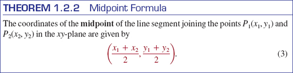
Midpoint Formula In Section 1.1 we saw that the midpoint of a line segment between two numbers a and b on the number line is the average, (a + b)/2. In the xy-plane, each coordinate of the midpoint M of a line segment joining two points P₁(x₁, y₁) and P₂(x₂, y₂), as shown in FIGURE 1.2.11, is the average of the corresponding coordinates of the endpoints of the intervals [x₁, x₂] and [y₁, y₂].

To prove this, we note in FIGURE 1.2.11 that triangles P₁CM and MDP₂ are congruent since corresponding angles are equal and d(P₁, M) = d(M, P₂). Hence, d(P₁, C) = d (M, D) or y − y₁ = y₂ − y. Solving the last equation for y gives . Similarly, d(C, M) = d(D, P₂) so that x − x₁ = x₂ − x and therefore . We summarize the result.

EXAMPLE 6 Midpoint of a Line Segment

Find the coordinates of the midpoint of the line segment joining A(–2, 5) and B(4, 1).

Solution From formula (3) the coordinates of the midpoint of the line segment joining the points A and B are given by

This point is indicated in red in FIGURE 1.2.12.

1.2 Exercises Answers to selected odd-numbered problems begin on page ANS-1.

In Problems 1-4, plot the given points.

1. (2, 3), (4, 5), (0, 2), (−1, −3)

2. (1, 4), (−3, 0), (−4, 2), (−1, −1)

3.

4. (0, 0.8), (−2, 0), (1.2,−1.2), (−2, 2)

In Problems 5-16, determine the quadrant in which the given point lies if (a, b) is in quadrant I.

5. (−a, b)

6. (a, − b)

7. (−a, −b)

8. (b, a)

9. (−b, a)

10. (−b, −a)

11. (a, a)

12. (b, −b)

13. (−a, −a)

14. (−a, a)

15. (b, −a)

16. (−b, b)

17. Plot the points given in Problems 5-16 if (a, b) is the point shown in FIGURE 1.2.13.

18. Give the coordinates of the points shown in FIGURE 1.2.14.

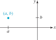
FIGURE 1.2.13 Point (a, b) in Problem 17

FIGURE 1.2.14 Points in Problem 18

19. The points (−2, 0), (−2, 6), and (3, 0) are vertices of a rectangle. Find the fourth vertex.

20. Describe the set of all points (x, x) in the coordinate plane. The set of all points (x, −x).

In Problems 21-26, sketch the set of points (x, y) in the xy-plane that satisfy the given conditions.

21. xy = 0

22. xy > 0

23. |x|≤1 and |y|≤2

24. x≤2 and y ≤ −1

25. |x| > 4

26. |y|≤1

In Problems 27-32, find the distance between the given points.

27. A(1, 2), B(−3, 4)

28. A(−1, 3), B(5, 0)

29. A(2, 4), B(−4, −4)

30. A(−12, −3), B(−5, −7)

31.

32.

In Problems 33-36, determine whether the points A, B, and C are vertices of a right triangle.

33. A(8, 1), B(−3, −1), C(10, 5)

34. A(−2, −1), B(8, 2), C(1, −11)

35. A(2, 8), B(0, −3), C(6, 5)

36. A(4, 0), B(1, 1), C(2, 3)

37. Determine whether the points A(0, 0), B(3, 4), and C(7, 7) are vertices of an isosceles triangle.

38. Find all points on the y-axis that are 5 units from the point (4, 4).

39. Consider the line segment joining A(−1, 2) and B(3, 4).

(a) Find an equation that expresses the fact that a point P(x, y) is equidistant from A and from B.

(b) Describe geometrically the set of points described by the equation in part (a).

40. Use the distance formula to determine whether the points A(−1, −5), B(2, 4), and C(4, 10) lie on a straight line.

41. Find all points with x-coordinate 6 such that the distance from each point to (–1, 2) is √85.

42. Which point, (1/√2, 1/√2)or (0.25, 0.97), is closer to the origin?

In Problems 43-48, find the midpoint of the line segment joining the points A and B.

43. A(4, 1), B(−2, 4)

44.

45. A(–1, 0), B(−8, 5)

46.

47. A(2a, 3b), B (4a, −6b)

48. A (x, x), B (−x, x + 2)

In Problems 49-52, find the point B if M is the midpoint of the line segment joining points A and B.

49.

50.

51. A(5, 8), M(−1, −1)

52. A(−10, 2), M(5, 1)

53. Find the distance from the midpoint of the line segment joining A(−1, 3) and B(3, 5) to the midpoint of the line segment joining C(4, 6) and D(−2, −10).

54. Find all points on the x-axis that are 3 units from the midpoint of the line segment joining (5, 2) and (−5, −6).

55. The x-axis is the perpendicular bisector of the line segment through A(2, 5) and B(x, y). Find x and y.

56. Consider the line segment joining the points A(0, 0) and B(6, 0). Find a point C(x, y) in the first quadrant such that A, B, and C are vertices of an equilateral triangle.

57. Find points P₁(x₁, y₁), P₂(x₂, y₂), and P₃(x₃, y₃) on the line segment joining A(3, 6) and B(5, 8) that divide the line segment into four equal parts.

Miscellaneous Applications

58. Going to Chicago Kansas City and Chicago are not directly connected by an interstate highway, but each city is connected to St. Louis and Des Moines. See FIGURE 1.2.15. Des Moines is approximately 40 mi east and 180 mi north of Kansas City, St. Louis is approximately 230 mi east and 40 mi south of Kansas City, and Chicago is approximately 360 mi east and 200 mi north of Kansas City. Assume that this part of the Midwest is a flat plane and that the connecting highways are straight lines. Which route from Kansas City to Chicago, through St. Louis or through Des Moines, is shorter?

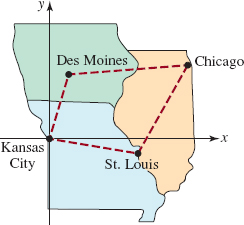
FIGURE 1.2.15 Map for Problem 58

For Discussion

59. The points A(1, 0), B(5, 0), C(4, 6), and D(8, 6) are vertices of a parallelogram. Discuss: How can it be shown that the diagonals of the parallelogram bisect each other? Carry out your ideas.

60. The points A(0, 0), B(a, 0), and C(a, b) are vertices of a right triangle. Discuss: How can it be shown that the midpoint of the hypotenuse is equidistant from the vertices? Carry out your ideas.

1.3 Circles and Graphs

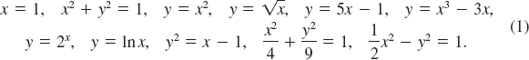
Introduction In Chapter 1 we studied equations as an equality of two algebraic quantities involving one variable. Our goal then was to find the solution set of the equation. In this and subsequent sections that follow we study equations in two variables, say x and y. Such an equation is simply a mathematical statement that asserts two quantities involving these variables are equal. In the fields of the physical sciences, engineering, and business, equations in two (or more) variables are a means of communication. For example, if a physicist wants to tell someone how far a rock dropped from a great height travels in a certain time t, he or she will write s = 16t². A mathematician will look at s = 16t² and immediately classify it as a certain type of equation. The classification of an equation carries with it information about properties shared by all equations of that kind. The remainder of this text is devoted to examining different kinds of equations involving two or more variables and studying their properties. Here is a sample of some of the equations in two variables that you will see:

Terminology A solution of an equation in two variables x and y is an ordered pair of numbers (a, b) that yields a true statement when x = a and y = b are substituted into the equation. For example, (−2, 4) is a solution of the equation y = x² because

is a true statement. We also say that the coordinates (−2, 4) satisfy the equation. As in Chapter 1, the set of all solutions of an equation is called its solution set. Two equations are said to be equivalent if they have the same solution set. For example, we will see in Example 4 of this section that the equation x² + y² + 10x − 2y + 17 = 0is equivalent to (x + 5)² + (y − 1)² = 3².

In the list given in (1), you might object that the first equation x = 1 does not involve two variables. It is a matter of interpretation! Because there is no explicit y dependence in the equation, the solution set of x = 1 can be interpreted to mean the set

The solutions of x = 1 are then ordered pairs (1, y), where you are free to choose y arbitrarily so long as it is a real number. For example, (1, 0) and (1, 3) are solutions of the equation x = 1. The graph of an equation is the visual representation in the rectangular coordinate system of the set of points whose coordinates (a, b) satisfy the equation. The graph of x = 1 is the vertical line shown in FIGURE 1.3.1.

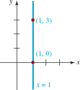
FIGURE 1.3.1 Graph of equation

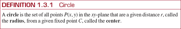
Circles The distance formula discussed in the preceding section can be used to define a set of points in the coordinate plane. One such important set is defined as follows.

If the center has coordinates C(h, k), then from the preceding definition a point P(x, y) lies on a circle of radius r if and only if

Since (x – h)² + (y – k)² is always nonnegative, we obtain an equivalent equation when both sides are squared. We conclude that a circle of radius r and center C(h, k) has the equation

In FIGURE 1.3.2 we have sketched a typical graph of an equation of the form given in (2). Equation (2) is called the standard form of the equation of a circle. We note that the symbols h and k in (2) represent real numbers and as such can be positive, zero, or negative. When h = 0, k = 0, we see that the standard form of the equation of a circle with center at the origin is

See FIGURE 1.3.3. When r = 1, we say that (2) or (3) is an equation of a unit circle. For example, x² + y² = lis an equation of a unit circle centered at the origin.

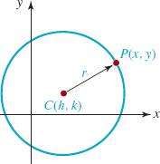
FIGURE 1.3.2 Circle with radius r and center (h, k)

FIGURE 1.3.3 Circle with radius r and center (0, 0)

EXAMPLE 1 Center and Radius

Find the center and radius of the circle whose equation is

Solution To obtain the standard form of the equation, we rewrite (4) as (x – 8)² + (y – (−2))² = 7².

Comparing this last form with (2) we identify h = 8, k = −2, and r = 7. Thus the circle is centered at (8, −2)and has radius 7.

EXAMPLE 2 Equation of a Circle

Find an equation of the circle with center C(− 5, 4) with radius √2.

Solution Substituting h = −5, k = 4, and r = √2 in (2) we obtain

(x − (−5))² + (y − 4)² = (√2)² or (x + 5)² + (y − 4)² = 2.

EXAMPLE 3 Equation of a Circle

Find an equation of the circle with center C(4, 3) and passing through P(1, 4).

Solution With h = 4 and k = 3, we have from (2)

FIGURE 1.3.4 Circle in Example 3

Since the point P(1, 4) lies on the circle as shown in FIGURE 1.3.4, its coordinates must satisfy equation (5). That is,

Thus the required equation in standard form is

Completing the Square If the terms (x – h)²and (y – k)²are expanded and the like terms grouped together, an equation of a circle in standard form can be written as

The terms in color added inside the parentheses on the left-hand side are also added to the right-hand side of the equality. This new equation is equivalent to (6).

Of course in this last form the center and radius are not apparent. To reverse the process, in other words, to go from (6) to the standard form (2), we must complete the square in both x and y. Recall from Section 1.3 that adding (a/2)² to a quadratic expression such as x² + ax yields x² + ax + (a/2)², which is the perfect square (x + a/2)². By rearranging the terms in (6),

and then adding (a/2)² and (b/2)² to both sides of the last equation

we obtain the standard form of the equation of a circle:

You should not memorize the last equation; we strongly recommend that you work through the process of completing the square each time.

EXAMPLE 4 Completing the Square

Find the center and radius of the circle whose equation is

Solution To find the center and radius we rewrite equation (7) in the standard form (2). First, we rearrange the terms,

Then, we complete the square in x and y by adding, in turn, (10/2)² in the first set of parentheses and (–2/2)² in the second set of parentheses. Proceed carefully here because we must add these numbers to both sides of the equation:

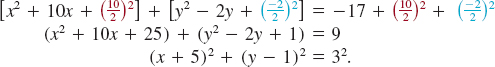
From the last equation we see that the circle is centered at (−5, 1) and has radius 3. See FIGURE 1.3.5.

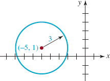
FIGURE 1.3.5 Circle in Example 4

It is possible that an expression for which we must complete the square has a leading coefficient other than 1. For example,

is an equation of a circle. As in Example 4 we start by rearranging the equation:

Now, however, we must do one extra step before attempting completion of the square; that is, we must divide both sides of the equation by 3 so that the coefficients of x² and y² are each 1:

At this point we can now add the appropriate numbers within each set of parentheses and to the right-hand side of the equality. You should verify that the resulting standard form is .

Semicircles If we solve (3) for y we get . This last expression is equivalent to the two equations . In like manner if we solve (3) for x we obtain . By convention, the symbol √ denotes a nonnegative quantity, thus the y-values defined by an equation such as are nonnegative. The graphs of the four equations highlighted in color are, in turn, the upper half, lower half, right half, and the left half of the circle shown in FIGURE 1.3.3. Each graph in FIGURE 1.3.6 is called a semicircle.

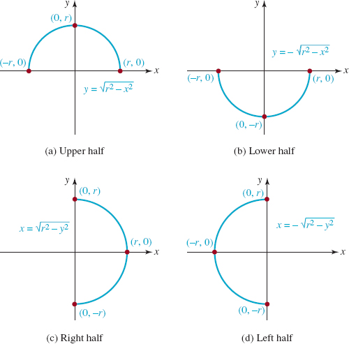
FIGURE 1.3.6 Semicircles

Inequalities One last point about circles. On occasion we encounter problems where we must sketch the set of points in the xy-plane whose coordinates satisfy inequalities such as x² + y² < r² or x² + y² ≥ r². The equation x² + y² = r² describes the set of points (x, y) whose distance to the origin (0, 0) is exactly r. Therefore, the inequality x² + y² < r² describes the set of points (x, y) whose distance to the origin is less than r. In other words, the points (x, y) whose coordinates satisfy the inequality x² + y² < r² are in the interior of the circle. Similarly, the points (x, y) whose coordinates satisfy x² + y² ≥ r² lie either on the circle or are exterior to it.

Graphs It is difficult to read a newspaper, read a science or business text, surf the Internet, or even watch the news on TV without seeing graphical representations of data. It may even be impossible to get past the first page in a mathematics text without seeing some kind of graph. So many diverse quantities are connected by means of equations and so many questions about the behavior of the quantities linked by the equation can be answered by means of a graph, that the ability to graph equations quickly and accurately—like the ability to do algebra quickly and accurately—is high on the list of skills essential to your success in a course in calculus. For the rest of this section we will talk about graphs in general, and more specifically, about two important aspects of graphs of equations.

Intercepts Locating the points at which the graph of an equation crosses the coordinates axes can be helpful when sketching a graph by hand. The x-intercepts of a graph of an equation are the points at which the graph crosses the x-axis. Since every point on the x-axis has y-coordinate 0, the x-coordinates of these points (if there are any) can be found from the given equation by setting y = 0 and solving for x. In turn, the y-intercepts of the graph of an equation are the points at which its graph crosses the y-axis. The y-coordinates of these points can be found by setting x = 0 in the equation and solving for y. See FIGURE 1.3.7.

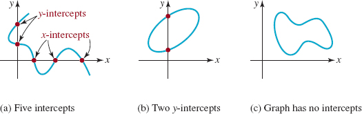
FIGURE 1.3.7 Intercepts of a graph

EXAMPLE 5 Intercepts

Find the intercepts of the graphs of the equations

(a) x² – y² = 9

(b) y = 2x² + 5x − 12.

Solution(a) To find the x-intercepts we set y = 0 and solve the resulting equation x² = 9 for x:

x² – 9 = 0 or (x + 3)(x – 3) = 0

gives x = −3 and x = 3. The x-intercepts of the graph are the points (−3, 0) and (3, 0). To find the y-intercepts we set x = 0 and solve -y² = 9 or y² = −9 for y. Because there are no real numbers whose square is negative we conclude the graph of the equation does not cross the y-axis.

(b) Setting y = 0 yields 2x² + 5x − 12 = 0. This is a quadratic equation and can be solved either by factoring or by the quadratic formula. Factoring gives

(x + 4)(2x − 3) = 0

and so x = –4 and . The x-intercepts of the graph are the points (–4, 0) and . Now, setting x = 0 in the equation y = 2x² + 5x – 12 immediately gives y = –12. The y-intercept of the graph is the point (0, −12).

EXAMPLE 6 Example 4 Revisited

Let's return to the circle in Example 4 and determine its intercepts from equation (7). Setting y = 0 in x² + y² + 10x − 2y + 17 = 0 and using the quadratic formula to solve x² + 10x+ 17 = 0 shows the x-intercepts of this circle are (–5 − 2√2, 0) and (−5 + 2√2, 0). If we let x = 0, then the quadratic formula shows that the roots of the equation y² – 2y + 17 = 0 are complex numbers. As seen in FIGURE 1.3.5, the circle does not cross the y-axis.

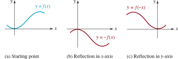
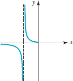
Symmetry A graph can also possess symmetry. You may already know that the graph of the equation y = x² is called a parabola. FIGURE 1.3.8 shows that the graph of y = x² is symmetric with respect to the y-axis since the portion of the graph that lies in the second quadrant is the mirror image or reflection of that portion of the graph in the first quadrant. In general, a graph is symmetric with respect to the y-axis if whenever (x, y) is a point on the graph, (−x, y) is also a point on the graph. Note in FIGURE 1.3.8 that the points (1, 1) and (2, 4) are on the graph. Because the graph possesses y-axis symmetry, the points (−1, 1) and (−2, 4) must also be on the graph. A graph is said to be symmetric with respect to the x-axis if whenever (x, y) is a point on the graph, (x, −y) is also a point on the graph. Finally, a graph is symmetric with respect to the origin if whenever (x, y) is on the graph, (−x, −y) is also a point on the graph. FIGURE 1.3.9 illustrates these three types of symmetries.

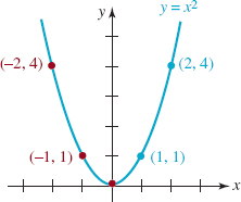
FIGURE 1.3.8 Graph with y-axis symmetry

FIGURE 1.3.9 Symmetries of a graph

Observe that the graph of the circle given in FIGURE 1.3.3 possesses all three of these symmetries.

As a practical matter we would like to know whether a graph possesses any symmetry in advance of plotting its graph. This can be done by applying the following tests to the equation that defines the graph.

The advantage of using symmetry in graphing should be apparent: If say, the graph of an equation is symmetric with respect to the x-axis, then we need only produce the graph for y ≥ 0 since points on the graph for y < 0 are obtained by taking the mirror images, through the x-axis, of the points in the first and second quadrants.

EXAMPLE 7 Test for Symmetry

By replacing x by -x in the equation y = x² and using (-x)² = x², we see that

y = (−x)² is equivalent to y = x².

This proves what is apparent in FIGURE 1.3.8; that is, the graph of y = x² is symmetric with respect to the y-axis.

EXAMPLE 8 Intercepts and Symmetry

Determine the intercepts and any symmetry for the graph of

Solution

Intercepts: Setting y = 0in equation (8) immediately gives x = 10. The graph of the equation has a single x-intercept, (10, 0). When x = 0, we get y² = 10, which implies that y = − √10; or y = √10. Thus there are two y-intercepts, (0, − √10) and (0, √10).

Symmetry: If we replace x by -x in the equation x + y² = 10, we get -x + y² = 10. This is not equivalent to equation (8). You should also verify that replacing x and y by -x and -y in (8) does not yield an equivalent equation. However, if we replace y by -y, we find that

x + (–y)² = 10 is equivalent to x + y² = 10.

Thus, the graph of the equation is symmetric with respect to the x-axis.

Graph: In the graph of the equation given in FIGURE 1.3.10 the intercepts are indicated and the x-axis symmetry should be apparent.

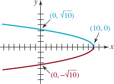
FIGURE 1.3.10 Graph of equation in Example 8

1.3 Exercises Answers to selected odd-numbered problems begin on page ANS-2.

In Problems 1-6, find the center and the radius of the given circle. Sketch its graph.

1. x² + y² = 5

2. x²+ y²=9

3. x² + (y − 3)² = 49

4. (x + 2)²+ y²=36

5.

6. (x + 3)²+ (y – 5)²= 25

In Problems 7-14, complete the square in x and y to find the center and the radius of the given circle.

7. x²+ y² + 8y = 0

8. x² + y² – 6x = 0

9. x² + y² + 2 x – 4y – 4 = 0

10. x² + y² – 18x – 6y – 10 = 0

11. x² + y² – 20x + 16y + 128 = 0

12. x² + y² + 3x – 16y + 63 = 0

13. 2x² + 2y² + 4x + 16y + 1 = 0

14.

In Problems 15-24, find an equation of the circle that satisfies the given conditions.

15. center (0, 0), radius 1

16. center (1, -3), radius 5

17. center (0, 2), radius

18. center (–9, -4), radius

19. endpoints of a diameter at (–1, 4) and (3, 8)

20. endpoints of a diameter at (4, 2) and (–3, 5)

21. center (0, 0), graph passes through (–1, -2)

22. center (4, -5), graph passes through (7, -3)

23. center (5, 6), graph tangent to the x-axis

24. center (–4, 3), graph tangent to the y-axis

In Problems 25-28, sketch the semicircle defined by the given equation.

25.

26.

27.

28.

29. Find an equation for the upper half of the circle x² + (y – 3)² = 4. The right half of the circle.

30. Find an equation for the lower half of the circle (x – 5)² + (y – 1)² = 9. The left half of the circle.

In Problems 31-34, sketch the set of points in the xy-plane whose coordinates satisfy the given inequality.

31. x² + y² ≥ 9

32. (x – 1)² + (y + 5)² ≤ 25

33. 1 ≤ x² + y² ≤ 4

34. x² + y² > 2y

In Problems 35 and 36, find the x- and y-intercepts of the given circle.

35. The circle with center (3, -6) and radius 7

36. The circle x² + y² + 5x – 6y = 0

In Problems 37-62, find any intercepts of the graph of the given equation. Determine whether the graph of the equation possesses symmetry with respect to the x-axis, y-axis, or origin. Do not graph.

37. y = -3x

38. y – 2x = 0

39. -x + 2y = 1

40. 2x + 3y = 6

41. x = y²

42. y = x³

43. y = x² – 4

44. x = 2y² – 4

45. y = x² – 2x – 2

46. y² = 16(x + 4)

47. y = x(x² – 3)

48. y = (x – 2)²(x + 2)²

49.

50. y³ – 4x² + 8 = 0

51. 4y² – x² = 36

52.

53.

54.

55.

56.

57. y = – 3

58.

59. y = |x – 9|

60. x = |y| – 4

61. |x| + |y| = 4

62. x + 3 = |y – 5|

In Problems 63-66, state all the symmetries of the given graph.

63.

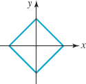
FIGURE 1.3.11 Graph for Problem 63

64.

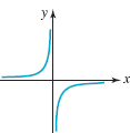
FIGURE 1.3.12 Graph for Problem 64

65.

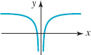
FIGURE 1.3.13 Graph for Problem 65

66.

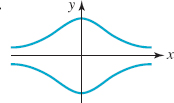
FIGURE 1.3.14 Graph for Problem 66

In Problems 67-72, use symmetry to complete the given graph.

>

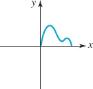
67. The graph is symmetric with respect to the y-axis.

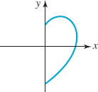
FIGURE 1.3.15 Graph for Problem 67

68. The graph is symmetric with respect to the x-axis.

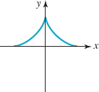
FIGURE 1.3.16 Graph for Problem 68

69. The graph is symmetric with respect to the origin.

FIGURE 1.3.17 Graph for Problem 69

70. The graph is symmetric with respect to the y-axis.

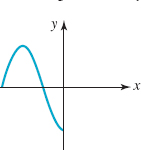
FIGURE 1.3.18 Graph for Problem 70

71. The graph is symmetric with respect to the x- and y-axes.

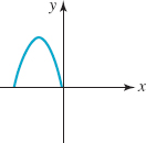
FIGURE 1.3.19 Graph for Problem 71

72. The graph is symmetric with respect to the origin.

FIGURE 1.3.20 Graph for Problem 72

For Discussion

FIGURE 1.3.21 Circles in Problem 74

73. Determine whether the following statement is true or false. Defend your answer.

If a graph has two of the three symmetries defined on page 19, then the graph must necessarily possess the third symmetry.

74. (a) The radius of the circle in FIGURE 1.3.21(a) is r. What is its equation in standard form?

(b)The center of the circle in FIGURE 1.3.21(b) is (h, k). What is its equation in standard form?

75. Discuss whether the following statement is true or false.

Every equation of the form x² + y² + ax + by + c = 0 is a circle.

1.4 Equations of Lines

Introduction Any pair of distinct points in the xy-plane determines a unique straight line. Our goal in this section is to find equations of lines. Fundamental to finding equations of lines is the concept of slope of a line.

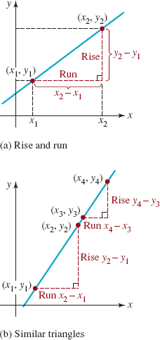
FIGURE 1.4.1 Slope of a line

Slope If P₁(x₁, y₁) and P₂(x₂, y₂) are two points such that x₁ ≠ x₂, then the number

is called the slope of the line determined by these two points. It is customary to call y₂ – y₁ the change in y or rise of the line; x₂ – x₁ is the change in x or the run of the line. Therefore, the slope (1) of a line is

See FIGURE 1.4.1(a). Any pair of distinct points on a line will determine the same slope. To see why this is so, consider the two similar right triangles in FIGURE 1.4.1(b). Since we know that the ratios of corresponding sides in similar triangles are equal we have

Hence the slope of a line is independent of the choice of points on the line.

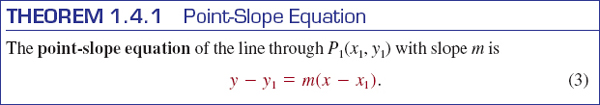
In FIGURE 1.4.2 we compare the graphs of lines with positive, negative, zero, and undefined slopes. In FIGURE 1.4.2(a) we see, reading the graph left to right, that a line with positive slope (m > 0) rises as x increases. FIGURE 1.4.2(b) shows that a line with negative slope (m < 0) falls as x increases. If P₁(x₁, y₁) and P₂(x₂, y₂) are points on a horizontal line, then y₁ = y₂ and so its rise is y₂ – y₁ = 0. Hence from (1) the slope is zero (m = 0). See FIGURE 1.4.2(c). If P₁(x₁, y₁) and P₂(x₂, y₂) are points on a vertical line, then x₁ = x₂ and so its run is x₂ – x₁ = 0. In this case we say that the slope of the line is undefined or that the line has no slope. See FIGURE 1.4.2(d).

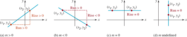
FIGURE 1.4.2 Lines with slope (a)-(c); line with no slope (d)

In general, since

it does not matter which of the two points is called P₁(x₁, y₁) and which is called P₂(x₂, y₂) in (1).

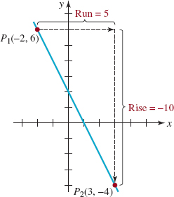
FIGURE 1.4.3 Line in Example 1

EXAMPLE 1: Slope and Graph

Find the slope of the line through the points (–2, 6) and (3, -4). Graph the line.

Solution Let (–2, 6) be the point P₁(x₁, y₁) and (3, -4) be the point P₂(x₂, y₂). The slope of the straight line through these points is

Thus the slope is -2, and the line through P₁ and P₂ is shown in FIGURE 1.4.3.

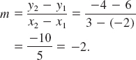
Point-Slope Equation We are now in a position to find an equation of a line L. To begin, suppose L has slope m and that P₁(x₁, y₁) is on the line. If P(x, y) represents any other point on L, then (1) gives

Multiplying both sides of the last equality by x – x₁ gives an important equation.

EXAMPLE 2: Point-Slope Equation

Find an equation of the line with slope 6 and passing through .

Solution Letting m = 6, x₁ = -, and y₁ = 2 we obtain from (3)

Simplifying gives

EXAMPLE 3: Point-Slope Equation

Find an equation of the line passing through the points (4, 3) and (–2, 5).

Solution First we compute the slope of the line through the points. From (1),

The point-slope equation (3) then gives

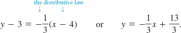
The distributive law a(b + c)= ab + ac is the source of many errors on students′ papers. A common error goes something like this: -2(2x – 3) = -2x – 3. The correct result is:

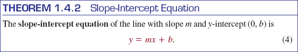
Slope-Intercept Equation Any line with slope (that is, any line that is not vertical) must cross the y-axis. If this y-intercept is (0, b), then with x₁ = 0, y₁ = b, the point-slope form (3) gives y – b = m(x – 0). The last equation simplifies to the next result.

FIGURE 1.4.4 Lines through the origin are y = mx

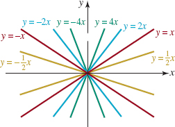
When b = 0in (4), the equation y = mx represents a family of lines that pass through the origin (0, 0). In FIGURE 1.4.4 we have drawn a few of the members of that family.

EXAMPLE 4: Example 3 Revisited

We can also use the slope-intercept form (4) to obtain an equation of the line through the two points in Example 3. As in that example, we start by finding the slope The equation of the line is then . By substituting the coordinates of either point (4, 3) or (–2, 5) into the last equation enables us to determine b. If we use x = 4 and y = 3, then and so . The equation of the line is .

Horizontal and Vertical Lines We saw in FIGURE 1.4.2(c) that a horizontal line has slope m = 0. An equation of a horizontal line passing through a point (a, b) can be obtained from (3), that is, y – b = 0(x – a) or y = b.

A vertical line through (a, b) has undefined slope and all points on the line have the same x-coordinate. The equation of a vertical line is then

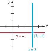
FIGURE 1.4.5 Horizontal and vertical lines in Example 5

EXAMPLE 5: Vertical and Horizontal Lines

Find equations for the vertical and horizontal lines through (3, -1). Graph these lines.

Solution Any point on the vertical line through (3, -1) has x-coordinate 3. The equation of this line is then x = 3. Similarly, any point on the horizontal line through (3, -1) has y-coordinate -1. The equation of this line is y = -1. Both lines are graphed in FIGURE 1.4.5.

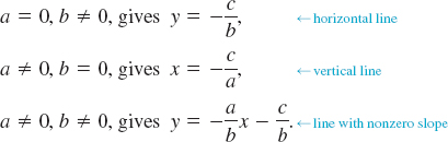
Linear Equation The equations (3), (4), (5), and (6) are special cases of the general linear equation in two variables x and y

where a and b are real constants and not both zero. The characteristic that gives (7) its name linear is that the variables x and y appear only to the first power. Observe that

EXAMPLE 6: Slope and y-intercept

Find the slope and the y-intercept of the line 3x – 7y + 5 = 0.

Solution We solve the linear equation for y:

Comparing the last equation with (4) we see that the slope of the line is and the y-intercept is .

If the x-and y-intercepts are distinct, the graph of the line can be drawn through the corresponding points on the x- and y-axes.

EXAMPLE 7: Graph of a Linear Equation

Graph the linear equation 3x – 2y + 8 = 0.

Solution There is no need to rewrite the linear equation in the form y = mx + b. We simply find the intercepts.

y-intercept: Setting x = 0 gives -2y + 8 = 0 or y = 4. The y-intercept is (0, 4).

x-intercept: Setting y = 0 gives 3x + 8 = 0 or x = -. The x-intercept is (, 0).

As shown in FIGURE 1.4.6, the line is drawn through the two intercepts (0, 4) and (, 0).

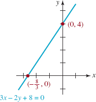
FIGURE 1.4.6 Line in Example 7

parallel lines

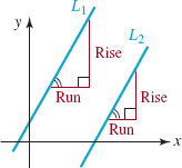
FIGURE 1.4.7 Parallel lines

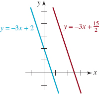
FIGURE 1.4.8 Parallel lines in Example 8

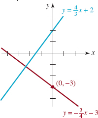
FIGURE 1.4.9 Perpendicular lines in Example 9

Parallel and Perpendicular Lines Suppose L₁ and L₂ are two distinct lines with slope. This assumption means that both L₁ and L₂ are nonvertical lines. Then necessarily L₁ and L₂ are either parallel or they intersect. If the lines intersect at a right angle they are said to be perpendicular. We can determine whether two lines are parallel or are perpendicular by examining their slopes.

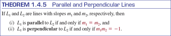
There are several ways of proving the two parts of Theorem 1.4.5. The proof of part (i) can be obtained using similar right triangles, as in FIGURE 1.4.7, and the fact that the ratios of corresponding sides in such triangles are equal. We leave the justification of part (ii) as an exercise. See Problems 49 and 50 in Exercises 1.4. Note that the condition m₁m₂ = -1 implies that m₂ = -1/m₁, that is, the slopes are negative reciprocals of each other. A horizontal line y = b and a vertical line x = a are perpendicular, but the latter is a line with no slope.

EXAMPLE 8: Parallel Lines

The linear equations 3x + y = 2 and 6x + 2y = 15 can be rewritten in the slope-intercept forms

respectively. As noted in color in the preceding line the slope of each line is -3. Therefore the lines are parallel. The graphs of these equations are shown in FIGURE 1.4.8.

EXAMPLE 9: Perpendicular Lines

Find an equation of the line through (0, -3) that is perpendicular to the graph of 4x – 3y + 6 = 0.

Solution We express the given linear equation in slope-intercept form:

4x – 3y + 6 = 0 implies 3y = 4x + 6.

Dividing by 3 gives y = x + 2. This line, whose graph is given in blue in FIGURE 1.4.9, has slope . The slope of any line perpendicular to it is the negative reciprocal of , namely, -. Since (0, —3) is the y-intercept of the required line, it follows from (4) that its equation is y = -x-3. The graph of the last equation is the red line in FIGURE 1.4.9.

1.4 Exercises: Answers to selected odd-numbered problems begin on page ANS-2.

In Problems 1-6, find the slope of the line through the given points. Graph the line through the points.

1. (3, -7), (1, 0)

2. (–4, -1), (1, -1)

3. (5, 2), (4, -3)

4. (1, 4), (6, -2)

5. (–1, 2), (3, -2)

6.

In Problems 7 and 8, use the graph of the given line to estimate its slope.

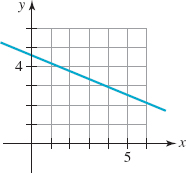
FIGURE 1.4.10 Graph for Problem 7

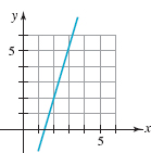
FIGURE 1.4.11 Graph for Problem 8

In Problems 9-16, find the slope and the x- and y-intercepts of the given line. Graph the line.

9. 3x – 4y + 12 = 0

10.

11. 2x – 3y = 9

12. -4x – 2y + 6 = 0

13. 2x + 5y – 8 = 0

14.

15.

16. y = 2x + 6

In Problems 17-22, find an equation of the line through (1, 2) with the indicated slope.

17.

18.

19. 0

20. -2

21. -1

22. undefined

In Problems 23-36, find an equation of the line that satisfies the given conditions.

23. Through (2, 3) and (6, -5)

24. Through (5, -6) and (4, 0)

25. Through (8, 1) and (–3, 1)

26. Through (2, 2) and (–2, -2)

27. Through (–2, 0) and (–2, 6)

28. Through (0, 0) and (a, b)

29. Through (–2, 4) parallel to 3x + y – 5 = 0

30. Through (1, -3) parallel to 2x – 5y + 4 = 0

31. Through (5, -7) parallel to the y-axis

32. Through the origin parallel to the line through (1, 0) and (–2, 6)

33. Through (2, 3) perpendicular to x – 4y + 1 = 0

34. Through (0, -2) perpendicular to 3x + 4y + 5 = 0

35. Through (–5, -4) perpendicular to the line through (1, 1) and (3, 11)

36. Through the origin perpendicular to every line with slope 2

In Problems 37-40, determine which of the given lines are parallel to each other and which are perpendicular to each other.

37. (a) 3x – 5y + 9 = 0

(b) 5x = – 3y

(c) -3x + 5y = 2

(d) 3x + 5y + 4 = 0

(e) -5x – 3y + 8 = 0

(f) 5x – 3y – 2 = 0

38. (a) 2x + 4y + 3 = 0

(b) 2x – y = 2

(c) x + 9 = 0

(d) x = 4

(c) y – 6 = 0

(d) -x – 2y + 6 = 0

39. (a) 3x – y – 1 = 0

(b) x – 3y + 9 = 0

(c) 3x + y = 0

(d)x + 3y = 1

(e) 6x – 3y + 10 = 0

(f) x + 2y = -8

40. (a) y + 5 = 0

(b) x = 7

(c) 4x + 6y = 3

(d) 12x – 9y + 7 = 0

(e)2x – 3y – 2 = 0

(f) 3x + 4y – 11 = 0

41. Find an equation of the line L shown in FIGURE 1.4.12 if an equation of the blue curve is y = x² + 1.

42. A tangent to a circle is defined to be a straight line that touches the circle at only one point P. Find an equation of the tangent line L shown in FIGURE 1.4.13.

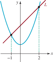
FIGURE 1.4.12 Graphs in Problem 41

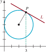
FIGURE 1.4.13 Circle and tangent line in Problem 42

For Discussion

43. How would you find an equation of the line that is the perpendicular bisector of the line segment through (, 10) and (, 4)?

44. Using only the concepts of this section, how would you prove or disprove that the triangle with vertices (2, 3), (–1, -3), and (4, 2) is a right triangle?

45. Using only the concepts of this section, how would you prove or disprove that the quadrilateral with vertices (0, 4), (–1, 3), (–2, 8), and (–3, 7) is a parallelogram?

46. If C is an arbitrary real constant, an equation such as 2x – 3y = C is said to define a family of lines. Choose four different values of C and plot the corresponding lines on the same coordinate axes. What is true about the lines that are members of this family?

47. Find the equations of the lines through (0, 4) that are tangent to the circle x² + y² = 4.

48. For the line ax + by + c = 0, what can be said about a, b, and c if

(a)the line passes through the origin,

(b)the slope of the line is 0,

(c)the slope of the line is undefined?

In Problems 49 and 50, to prove part (ii) of Theorem 1.4.5 you have to prove two things, the only if part (Problem 49) and then the if part (Problem 50) of the theorem.

49. In FIGURE 1.4.14, without loss of generality, we have assumed that two perpendicular lines y = m₁x, m₁ > 0, and y = m₂x, m₂ < 0, intersect at the origin. Use the information in the figure to prove the only if part:

If L₁ and L₂ are perpendicular lines with slopes m₁ and m₂, then m₁m₂ = -1.

50. Reverse your argument in Problem 49 to prove the if part:

If L₁ and L₂ are lines with slopes m₁ and m₂ such that m₁m₂ = -1, then L₁ and L₂ are perpendicular.

FIGURE 1.4.14 Lines through origin in Problems 49 and 50

1.5 Functions and Graphs

Introduction Using the objects and the persons around us, it is easy to make up a rule of correspondence that associates, or pairs, the members, or elements, of one set with the members of another set. For example, to each social security number there is a person, to each car registered in the state of California there is a license plate number, to each book there corresponds at least one author, to each state there is a governor, and so on. A natural correspondence occurs between a set of 20 students and a set of, say, 25 desks in a classroom when each student selects and sits in a different desk. In mathematics we are interested in a special type of correspondence, a single-valued correspondence, called a function.

The set Y is not necessarily the range

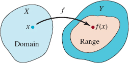
FIGURE 1.5.1 Domain and range of a function f

In the student/desk correspondence above suppose the set of 20 students is the set X and the set of 25 desks is the set Y. This correspondence is a function from the set X to the set Y provided no student sits in two desks at the same time.

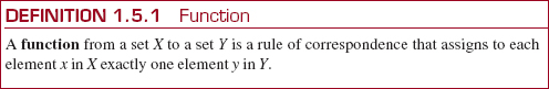
Terminology A function is usually denoted by a letter such as f, g, or h. We can then represent a function f from a set X to a set Y by the notation f : x → Y. The set X is called the domain of f. The set of corresponding elements y in the set Y is called the range of the function. For our student/desk function, the set of students is the domain and the set of 20 desks actually occupied by the students constitutes the range. Notice that the range of f need not be the entire set Y. The unique element y in the range that corresponds to a selected element x in the domain X is called the value of the function at x, or the image of x, and is written f(x). The latter symbol is read “f of x” or “f at x,” and we write y = f(x). See FIGURE 1.5.1. In many texts, x is also called the input of the function f and the value f(x) is called the output of f. Since the value of y depends on the choice of x, y is called the dependent variable; x is called the independent variable. Unless otherwise stated, we will assume hereafter that the sets X and Y consist of real numbers.

EXAMPLE 1: The Squaring Function

The rule for squaring a real number is given by the equation y = x² or f(x) = x². The values of f at x = -5 and x = are obtained by replacing x, in turn, by the numbers -5 and :

Occasionally for emphasis we will write a function using parentheses in place of the symbol x. For example, we can write the squaring function f(x) = x² as

This illustrates the fact that x is a placeholder for any number in the domain of the function y = f(x). Thus, if we wish to evaluate (1) at, say, 3 + h, where h represents a real number, we put 3 + h into the parentheses and carry out the appropriate algebra:

See (3) of Section R.6.

If a function f is defined by means of a formula or an equation, then typically the domain of y = f(x) is not expressly stated. We will see that we can usually deduce the domain of y = f(x) either from the structure of the equation or from the context of the problem.

EXAMPLE 2: Domain and Range

In Example 1, since any real number x can be squared and the result x² is another real number, f(x) = x² is a function from R to R, that is, f: R → R. In other words, the domain of f is the set R of real numbers. Using interval notation, we also write the domain as (–∞, ∞).The range offis the set of nonnegative real numbers or [0, ∞); this follows from the fact that x² ≥ 0 for every real number x.

Domain of a Function As mentioned earlier, the domain of a function y = f(x) that is defined by a formula is usually not specified. Unless stated or implied to the contrary, it is understood that

The domain of a function f is the largest subset of the set of real numbers for which f(x) is a real number.

This set is sometimes referred to as the implicit domain of the function. For example, we cannot compute f(0) for the reciprocal function f(x) = 1/x since 1/0 is not a real number. In this case we say that f is undefined at x = 0. Since every nonzero real number has a reciprocal, the domain of f(x) = 1/x is the set of real numbers except 0. By the same reasoning, the function g(x) = 1/(x² – 4) is not defined at either x = -2 or x = 2, and so its domain is the set of real numbers with the numbers -2 and 2 excluded. The square root function h(x) = is not defined at x = -1 because is not a real number. In order for h(x) = to be defined in the real number system we must require the radicand, in this case simply x, to be nonnegative. From the inequality x ≥ 0 we see that the domain of the function h is the interval [0,∞).

EXAMPLE 3: Domain and Range

Determine the domain and range of .

Solution The radicand x – 3 must be nonnegative. By solving the inequality x – 3 ≥ 0 we get x ≥ 3, and so the domain of f is [3, ∞). Now, since the symbol denotes the principal square root of a number, ≥ 0 for x ≥ 3 and consequently 4 + ≥ 4. The smallest value of f(x) occurs at x = 3 and is f(3) = 4 + = 4. Moreover, because x – 3 and increase as x takes on increasingly larger values, we conclude that y ≥ 4. Consequently the range of f is [4, ∞).

In most cases it is not easy to determine the range by inspection of a function defined by a formula.

EXAMPLE 4: Domains of Two Functions

Determine the domain of

Solution A function that is given by a fractional expression is not defined at the x-values for which its denominator is equal to 0.

Since the denominator of f(x) factors, x² – 3x – 4 = (x + 1)(x – 4), we see that (x + 1)(x – 4) = 0 for x = -1 and x = 4. These are the only numbers for which f is not defined. Hence, the domain of the function f is the set of real numbers with x = -1 and x = 4 excluded.

Using interval notation, the domain of the function f in part (b) of Example 4 can be written as

As an alternative to this ungainly union of disjoint intervals, this domain can also be written using set-builder notation as {x | x real, x ≠ -1 and x = 4}.

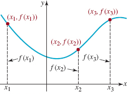
FIGURE 1.5.2 Points on the graph of an equation y = f(x)

Graphs A function is often used to describe phenomena in fields such as science, engineering, and business. In order to interpret and utilize data, it is useful to display this data in the form of a graph. The graph of a function f is the graph of the set of ordered pairs (x, f(x)), where x is in the domain of f. In the xy-plane an ordered pair (x, f(x)) is a point, so that the graph of a function is a set of points. If a function is defined by an equation y = f(x), then the graph of f is the graph of the equation. To obtain points on the graph of an equation y = f(x), we judiciously choose numbers x₁, x₂, x₃,…in its domain, compute f(x₁), f(x₂), f (x₃),…, plot the corresponding points (x₁, f(x₁)), (x₂, f(x₂)), (x₃, f(x₃)),…and then connect these points with a curve. See FIGURE 1.5.2. Keep in mind that

a value of x is a directed distance from the y-axis, and

a function value f(x) is a directed distance from the x-axis.

End Behavior A word about the figures in this text is in order. With a few exceptions, it is usually impossible to display the complete graph of a function, and so we often display only the more important features of the graph. In FIGURE 1.5.3(a), notice that the graph goes down on its left and right sides. Unless indicated to the contrary, we may assume that there are no major surprises beyond what we have shown and the graph simply continues in the manner indicated. The graph in FIGURE 1.5.3(a) indicates the so-called end behavior or global behavior of the function: For a point (x, y) on the graph, the values of the y-coordinate become unbounded in magnitude in the downward or negative direction as the x-coordinate becomes unbounded in magnitude in both the negative and positive directions on the number line. It is convenient to describe this end behavior using the symbols

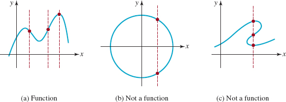
FIGURE 1.5.3 Vertical line test

The arrow symbol → in (2) is read “approaches.” Thus, for example, y → -∞” as x → ∞” is read “y approaches negative infinity as x approaches infinity.”

If a graph terminates at either its right or left end, we will indicate this by a dot when clarity demands it. See FIGURE 1.5.4. We will use a solid dot to represent the fact that the endpoint is included on the graph and an open dot to signify that the endpoint is not included on the graph.

Vertical Line Test From the definition of a function we know that for each x in the domain of f there corresponds only one value f(x) in the range. This means a vertical line that intersects the graph of a function y = f(x) (this is equivalent to choosing an x) can do so in at most one point. Conversely, if every vertical line that intersects a graph of an equation does so in at most one point, then the graph is the graph of a function. The last statement is called the vertical line test for a function. See FIGURE 1.5.3(a). On the other hand, if some vertical line intersects a graph of an equation more than once, then the graph is not that of a function. See FIGURES 1.5.3(b) and 1.5.3(c). When a vertical line intersects a graph in several points, the same number x corresponds to different values of y in contradiction to the definition of a function.

If you have an accurate graph of a function y = f(x), it is often possible to see the domain and range off. In FIGURE 1.5.4 assume that the colored curve is the entire, or complete, graph of some function f. The domain off then is the interval [a, b] on the x-axis and the range is the interval [c, d] on the y-axis.

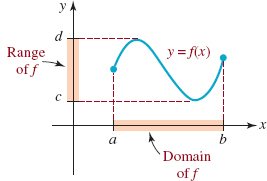
FIGURE 1.5.4 Domain and range interpreted graphically

EXAMPLE 5 Example 3 Revisited

From the graph of given in FIGURE 1.5.5, we can see that the domain and range of fare, respectively, [3, ∞) and [4, ∞). This agrees with the results in Example 3.

As shown in FIGURE 1.5.3(b), a circle is not the graph of a function. Actually, an equation such as x² + y² = 9 defines (at least) two functions of x. If we solve this equation for y in terms of x we get y = ± Because of the single-valued convention for the symbol, both equations y = and y = – define functions. As we saw in Section 2.2, the first equation defines an upper semicircle and the second defines a lower semicircle. From the graphs shown in FIGURE 1.5.6, the domain of is [-3, 3] and the range is [0, 3]; the domain and range of y = – are [-3, 3] and [-3, 0], respectively.

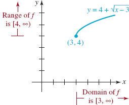
FIGURE 1.5.5 Graph of function f in Example 5

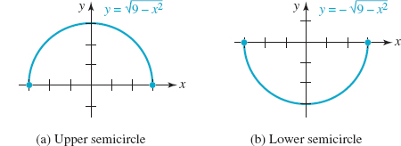
FIGURE 1.5.6 These semicircles are graphs of functions

Intercepts To graph a function defined by an equation y = f(x), it is usually a good idea to first determine whether the graph of f has any intercepts. Recall that all points on the y-axis are of the form (0, y). Thus, if 0 is in the domain of a function f, the y-intercept is the point on the y-axis whose y-coordinate is f(0), in other words, (0, f(0)). See FIGURE 1.5.7(a). Similarly, all points on the x-axis have the form (x, 0). This means that to find the x-intercepts of the graph of y = f(x), we determine the values of x that make y = 0. That is, we must solve the equation f(x) = 0 for x. A number c for which

is referred to as either a zero of the function f or a root (or solution) of the equation f(x) = 0. The real zeros of a function f are the x-coordinates of the x-intercepts of the graph of f. In FIGURE 1.5.7(b), we have illustrated a function that has three zeros x₁, x₂, and x₃ because f(x₁) = 0, f(x₂) = 0, and f(x₃) = 0. The corresponding three x-intercepts are the points (x₁, 0), (x₂, 0), and (x₃, 0). Of course, the graph of the function may have no intercepts. This is illustrated in FIGURE 1.5.5.

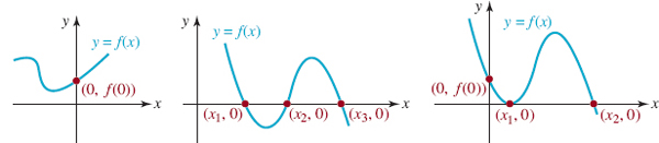
FIGURE 1.5.7 Intercepts of the graph of a function f

A graph does not necessarily have to cross a coordinate axis at an intercept, a graph could simply be tangent to, or touch, an axis. In FIGURE 1.5.7(c) the graph of y = f(x) is tangent to the x-axis at (x₁, 0). Also, the graph of a function f can have at most one y-intercept since, if 0 is the domain of f, there can correspond only one y-value, namely, y = f(0).

EXAMPLE 6: Intercepts

Find, if possible, the x- and y-intercepts of the given function.

(a)f(x) = x² + 2x – 2

(b)

Solution (a) Since 0 is in the domain of f, f(0) = -2 is the y-coordinate of the y-intercept of the graph of f. The y-intercept is the point (0,-2). To obtain the x-intercepts we must determine whether f has any real zeros, that is, real solutions of the equation f(x) = 0. Since the left-hand side of the equation x² + 2x – 2 = 0 has no obvious factors, we use the quadratic formula to obtain . Since the zeros off are the numbers 1 – and 1 + . The x-intercepts are the points (1 – , 0) and (1 + , 0).

(b) Because 0 is not in the domain of f(f(0) = -3/0 is not defined), the graph of f possesses no y-intercept. Now since f is a fractional expression, the only way we can have f(x) = 0 is to have the numerator equal zero. Factoring the left-hand side of x² – 2x – 3 = 0 gives (x + 1)(x – 3) = 0. Therefore the numbers -1 and 3 are the zeros of f. The x-intercepts are the points (– 1, 0) and (3, 0).

Approximating Zeros Even when it is obvious that the graph of a function y = f(x) possesses x-intercepts it is not always a straightforward matter to solve the equation f(x) = 0. In fact, it is impossible to solve some equations exactly; sometimes the best we can do is to approximate the zeros of the function. One way of doing this is to 4 We will study another way of approximat-obtain a very accurate graph of f.

We will study another way of approximating zeros of a function in Section 4.5.

EXAMPLE 7: Intercepts

With the aid of a graphing utility the graph of the function f(x) = x³ – x + 4 is given in FIGURE 1.5.8. From f(0) = 4 we see that the y-intercept is (0, 4). As we see in the figure, there appears to be only one x-intercept with its x-coordinate close to -1.7 or -1.8. But there is no convenient way of finding the exact values of the roots of the equation x³ – x + 4 = 0. We can, however, approximate the real root of this equation with the aid of the find root feature of either a graphing calculator or computer algebra system. We find that x ≈ -1.796and so the approximate x-intercept is (–1.796, 0).As a check, note that the function value

is nearly 0.

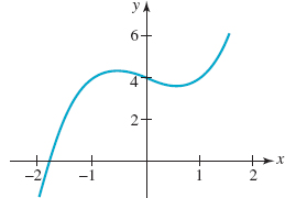
FIGURE 1.5.8 Approximate x-intercept in Example 7

1.5 Exercises: Answers to selected odd-numbered problems begin on page ANS-3.

In Problems 1-6, find the indicated function values.

1. If f(x) = x² – 1; f(–5), f(), f(3), and f(6)

2. If f(x) = -2x² + x;

3. If f(x) = f(–1), f(0), f(3), and f(5)

4.

5.

6.

In Problems 7 and 8, find

for the given function f and simplify as much as possible.

7. f() = -2()² + 3()

8. f() = ()³ – 2()² + 20

9. For what values of x is f(x) = 6x² – 1 equal to 23?

10. For what values of x is equal to 4?

In Problems 11-20, find the domain of the given function f.

11.

12.

13.

14.

15.

16.

17.

18.

19.

20.

In Problems 21-24, determine whether the graph in the figure is the graph of a function.

21.

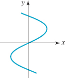
FIGURE 1.5.9 Graph for Problem 21

22.

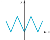
FIGURE 1.5.10 Graph for Problem 22

23.

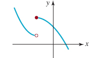
FIGURE 1.5.11 Graph for Problem 23

24.

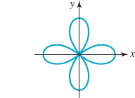
FIGURE 1.5.12 Graph for Problem 24

In Problems 25-28, use the graph of the function f given in the figure to find its domain and range.

25.

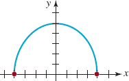
FIGURE 1.5.13 Graph for Problem 25

26.

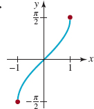
FIGURE 1.5.14 Graph for Problem 26

27.

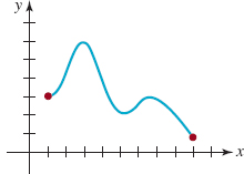
FIGURE 1.5.15 Graph for Problem 27

28.

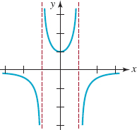
FIGURE 1.5.16 Graph for Problem 28

In Problems 29-36, find the zeros of the given function f.

29. f(x) = 5x + 6

30. f(x) = -2x + 9

31. f(x) = x² – 5x + 6

32. f(x) = x² – 2x – 1

33. f(x) = x(3x – 1)(x + 9)

34. f(x) = x³ – x² – 2x

35. f(x) = x⁴ – 1

36.

In Problems 37-44, find the x- and y-intercepts, if any, of the graph of the given function f. Do not graph.

37.

38. f(x) = x² – 6x + 5

39. f(x) = 4(x – 2)² – 1

40. f(x) = (2x – 3)(x² + 8x + 16)

41.

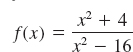
42.

43.

44.

In Problems 45 and 46, find two functions y = f₁(x) and y = f₂(x) defined by the given equation. Find the domain of the functions f₁ and f₂.

45. x = y² – 5

46. x² – 4y² = 16

In Problems 47 and 48, use the graph of the function f given in the figure to estimate the values of f(– 3), f(– 2), f(–1), f(1), f(2), and f(3). Estimate the y-intercept.

47.

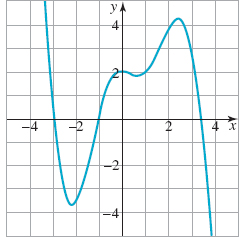
FIGURE 1.5.17 Graph for Problem 47

48.

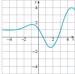
FIGURE 1.5.18 Graph for Problem 48

In Problems 49 and 50, use the graph of the function f given in the figure to estimate the values of f(–2), f(–1.5), f(0.5), f(1), f(2), and f(3.2). Estimate the x-intercepts.

49.

FIGURE 1.5.19 Graph for Problem 49

50.

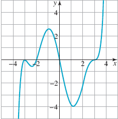
FIGURE 1.5.20 Graph for Problem 50

51. Factorial Function In your study of mathematics some of the functions that you will encounter have as their domain the set of positive integers n. The factorial function f(n) = n! is defined as the product of the first n positive integers, that is,

(a) Evaluate f(2), f(3), f(5), and f(7).

(b) Show that f(n + 1) = f(n) · (n + 1).

(c) Simplify f(n + 2)/f(n).

52. A Sum Function Another function of a positive integer n gives the sum of the first n squared positive integers:

(a) Find the value of the sum 1² + 2² +…+ 99² + 100².

(b) Find n such that 300 < S(n) < 400. [Hint: Use a calculator.]

For Discussion

53. Determine an equation of a function y = f(x) whose domain is (a) [3, ∞),

(b) (3, ∞).

54. Determine an equation of a function y = f(x) whose range is

(a) [3, ∞), (b) (3, ∞).

55. What is the only point that can be both an x- and a y-intercept for the graph of a function y = f(x)?

56. Consider the function . After factoring the denominator and canceling a common factor we can write . Discuss: Is x = 1 in the domain of ?

1.6 Symmetry and Transformations

Introduction In this section we discuss two aids in sketching graphs of functions quickly and accurately. If you determine in advance that the graph of a function possesses symmetry, then you can cut your work in half. In addition, sketching a graph of a complicated-looking function is expedited if you recognize that the required graph is actually a transformation of the graph of a simpler function. This latter graphing aid is based on your prior knowledge of the graphs of some basic functions.

Power Functions A function of the form

where n represents a real number is called a power function. The domain of a power function depends on the power n. For example, we have already seen in Section 1.5 for n = 2, n = , and n = -1, respectively, that

the domain of f(x) = x² is the set R of real numbers or (–∞, ∞),

the domain of f(x) = x^1/2 = is [0, ∞), and

the domain of is the set R of real numbers except x = 0.

Simple power functions, or modified versions of these functions, occur so often in problems that you do not want to spend valuable time plotting their graphs. We suggest that you know (memorize) the short catalogue of graphs of power functions given in FIGURE 1.6.1. You already know that the graph in part (a) of that figure is a line and may know that the graph in part (b) is called a parabola.

Symmetry In Section 1.3 we discussed symmetry of a graph with respect to the y-axis, the x-axis, and the origin. Of those three types of symmetries, the graph of a function can be symmetric with respect to the y-axis or with respect to the origin, but the graph of a nonzero function cannot be symmetric with respect to the x-axis. See Problem 43 in Exercises 1.6. If the graph of a function is symmetric with respect to the y-axis, then as we know the points (x, y) and (–x, y) are on the graph of f. Similarly, if the graph of a function is symmetric with respect to the origin, the points (x, y) and (–x, -y) are on its graph. For functions, the following two tests for symmetry are equivalent to tests (i) and (ii), respectively, on page 20.

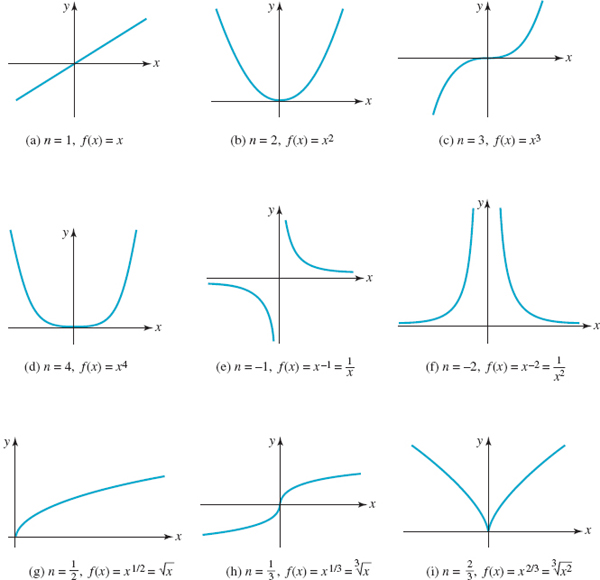
FIGURE 1.6.1 Brief catalogue of power functions f (x) =xⁿ for various n

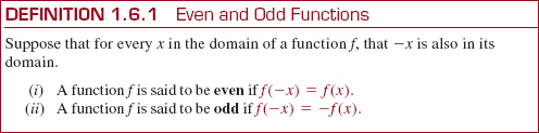
FIGURE 1.6.2 Even function

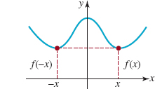
In FIGURE 1.6.2, observe that if f is an even function and

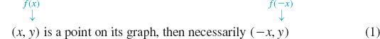
is also on its graph. Similarly we see in FIGURE 1.6.3 that iff is an odd function and

is on its graph. We have proved the following result.

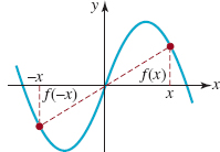
FIGURE 1.6.3 Odd function

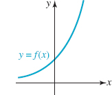
FIGURE 1.6.4 Function is neither odd nor even

Inspection of FIGURES 1.6.2 and 1.6.3 shows that the graphs, in turn, are symmetric with respect to the y-axis and origin. The function whose graph is given in FIGURE 1.6.4 is neither even nor odd, and so its graph possesses no y-axis or origin symmetry.

In view of Definition 1.6.1 and Theorem 1.6.1 we can determine symmetry of a graph of a function in an algebraic manner.

EXAMPLE 1 Odd and Even Functions

(a) f(x) = x³is an odd function since by Definition 1.6.1(ii),

This proves what we see in FIGURE 1.6.1(c), the graph of f (x) = x³ is symmetric with respect to the origin. For example, since f(1) = 1, (1, 1) is a point on the graph of y = x³. Because f is an odd function, f(–1) = -f(1) implies (–1,-1) is on the same graph.

(b) f(x) = xis an even function since by Definition 1.6.1(i) and the laws of exponents

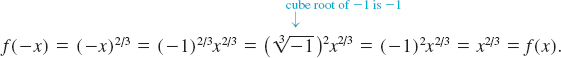
In FIGURE 1.6.1(i), we see that the graph of f is symmetric with respect to the y-axis. For example, since f(8) = 8 = 4, (8, 4) is a point on the graph of y = x. Because f is an even function, f(–8) = f(8) implies (–8, 4) is also on the same graph.

(c) f(x) = x³ + 1 is neither even nor odd. From

we see that f(–x) ≠ f(x), and f(–x) ≠ -f(x). Hence the graph of f is neither symmetric with respect to the y-axis nor symmetric with respect to the origin.

The graphs in FIGURE 1.6.1, with part (g) the only exception, possess either y-axis or origin symmetry. The functions in FIGURES 1.6.1(b), (d), (f), and (i) are even, whereas the functions in FIGURES 1.6.1(a), (c), (e), and (h) are odd.

Often we can sketch the graph of a function by applying a certain transformation to the graph of a simpler function (such as those given in FIGURE 1.6.1). We will consider two kinds of graphical transformations, rigid and nonrigid.

Rigid Transformations A rigid transformation of a graph is one that changes only the position of the graph in the xy-plane but not its shape. For example, the circle (x – 2)² + (y – 3)² = 1 with center (2, 3) and radius r = 1, has exactly the same shape as the circle x² + y² = 1 with center at the origin. Thus we can think of the graph of (x – 2)² + (y – 3)² = 1 as the graph of x² + y² = 1 shifted horizontally 2 units to the right followed by an upward vertical shift of 3 units. For the graph of a function y = f(x) we examine four kinds of shifts or translations.

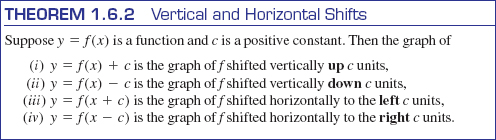
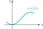
FIGURE 1.6.5 Graph of y = f (x)

Consider the graph of a function y = f (x) given in FIGURE 1.6.5. The shifts of this graph described in (i)-(iv) of Theorem 1.6.2 are the graphs in red in parts (a)-(d) of FIGURE 1.6.6. If (x, y) is a point on the graph of y = f (x) and the graph of f is shifted, say, upward by c > 0 units, then (x, y + c) is a point on the new graph. In general, the x-coordinates do not change as a result of a vertical shift. See FIGURES 1.6.6(a) and 1.6.6(b). Similarly, in a horizontal shift the y-coordinates of points on the shifted graph are the same as on the original graph. See FIGURES 1.6.6(c) and 1.6.6(d).

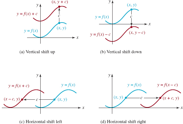
FIGURE 1.6.6 Vertical and horizontal shifts of the graph of y = f (x) by an amount c > 0.

EXAMPLE 2: Vertical and Horizontal Shifts

The graphs of y = x² + 1, y = x² – 1, y = (x + 1)², and y = (x – 1)² are obtained from the blue graph of f(x) = x² in FIGURE 1.6.7(a) by shifting this graph, in turn, 1 unit up (FIGURE 1.6.7(b)), 1 unit down (FIGURE 1.6.7(c)), 1 unit to the left (FIGURE 1.6.7(d)), and 1 unit to the right (FIGURE 1.6.7(e)).

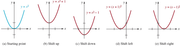
FIGURE 1.6.7 Shifted graphs in red in Example 2

Combining Shifts In general, the graph of a function

where c₁ and c₂ are positive constants, combines a horizontal shift (left or right) with a vertical shift (up or down). For example, the graph of y = f(x – c₁) + c₂ is the graph of y = f(x) shifted c₁ units to the right and then c₂ units up.

EXAMPLE 3: Graph Shifted Horizontally and Vertically

Graph y = (x + 1)² – 1.

Solution From the preceding paragraph we identify in (3) the form y = f (x + c₁) – c₂ with c₁ = 1 and c₂ = 1. Thus, the graph of y = (x + 1)² – 1 is the graph of f(x) = x² shifted 1 unit to the left followed by a downward shift of 1 unit. The graph is given in FIGURE 1.6.8.

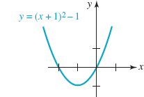
FIGURE 1.6.8 Shifted graph in Example 3

From the graph in FIGURE 1.6.8 we see immediately that the range of the function y = (x + 1)² – 1 = x² + 2x is the interval [-1, ∞) on the y-axis. Note also that the graph has x-intercepts (0, 0) and (–2, 0); you should verify this by solving x² + 2x = O. Also, if you reexamine FIGURE 1.5.5 in Section 1.5 you will see that the graph of is the graph of the square root function f(x) = √x (FIGURE 1.6.1(g)) shifted 3 units to the right and then 4 units up.

Another way of rigidly transforming a graph of a function is by a reflection in a coordinate axis.

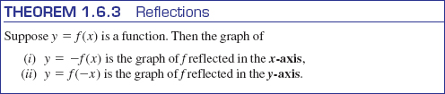
In part (a) of FIGURE 1.6.9 we have reproduced the graph of a function y = f(x) given in FIGURE 1.6.5. The reflections of this graph described in parts (i) and (ii) of Theorem 1.6.3 are illustrated in FIGURES 1.6.9(b) and 1.6.9(c). If (x, y) denotes a point on the graph of y = f(x), then the point (x, -y) is on the graph of y = -f(x) and (–x, y) is on the graph of y = f (–x). Each of these reflections is a mirror image of the graph of y = f(x) in the respective coordinate axis.

Reflection or mirror image

FIGURE 1.6.9 Reflections in the coordinate axes