![]()
Integration with R
This chapter will introduce R and show how it is integrated with Microsoft Azure Machine Learning. Through simple examples, you will learn how to write and run your own R code when working with Azure Machine Learning. You will also learn the R packages supported by Azure Machine Learning, and how you can use them in the Azure Machine Learning Studio (ML Studio).
R in a Nutshell
R is an open source statistical programming language that is commonly used by the computational statistics and data science community for solving an extensive spectrum of business problems. These problems span the following areas:
- Bioinformatics (e.g. genome analysis)
- Actuarial sciences (e.g. figuring out risk exposures for insurance, finance, and other industries)
- Telecommunication (analyzing churn in corporate and consumer customer base, fraudulent SIM card usage, or mobile usage patterns)
- Finance and banking (e.g. identifying fraud in financial transactions), manufacturing (e.g. predicting hardware component failure times), and many more.
When using R, users feel empowered by its toolbox of R packages that provides powerful capabilities for data analysis, visualization, and modeling. As of 2014, the Comprehensive R Archive Network (CRAN) provides a large collection of more than 5000 R packages. Besides CRAN, there are many other R packages available on Github (https://github.com/trending?l=r) and specialized R packages for bioinformatics in the Bioconductor R repository (www.bioconductor.org/).
![]() Note R was created at the University of Auckland by Joss Ihaka and Robert Gentleman in 1994. Since R’s creation, many leading computer scientists and statisticians have fueled R’s success by contributing to the R codebase or providing R packages that enable R users to leverage the latest techniques for statistical analysis, visualization, and data mining. This has propelled R to become one of the languages for data scientists. Learn more about R at www.r-project.org/.
Note R was created at the University of Auckland by Joss Ihaka and Robert Gentleman in 1994. Since R’s creation, many leading computer scientists and statisticians have fueled R’s success by contributing to the R codebase or providing R packages that enable R users to leverage the latest techniques for statistical analysis, visualization, and data mining. This has propelled R to become one of the languages for data scientists. Learn more about R at www.r-project.org/.
Given the momentum in the data science community in using R to tackle machine learning problems, it is super important for a cloud-based machine learning platform to empower data scientists to continue using the familiar R scripts that they have written, and continue to be productive. Currently, more than 400 R packages are supported by Azure Machine Learning. Table 3-1 shows a subset of the R packages currently supported. These R packages enable you to model a wide spectrum of machine learning problems from market basket analysis, classification, regression, forecasting, and visualization.
Table 3-1. R Packages Supported by Azure Machine Learning
|
R packages |
Description |
|---|---|
|
Arules |
Frequent itemsets and association rule mining |
|
FactoMineR |
Data exploration |
|
Forecast |
Univariate time series forecasts (exponential smoothing and automatic ARIMA) |
|
ggplot2 |
Graphics |
|
Glmnet |
Linear regression, logistics and multinomial regression models, poisson regression, and Cox Model |
|
Party |
Tools for decision tree |
|
randomForest |
Classification and regression models based on a forest of trees |
|
Rsonlp |
General non-linear optimization using augmented lagrange multipliers |
|
Xts |
Time series |
|
Zoo |
Time series |
![]() Tip To get the complete list of installed packages, create a new experiment in Cloud Machine Learning, use the Execute R Script module, provide the following script in the body of the Execute R Script module, and run the experiment. After the experiment
Tip To get the complete list of installed packages, create a new experiment in Cloud Machine Learning, use the Execute R Script module, provide the following script in the body of the Execute R Script module, and run the experiment. After the experiment
out <- data.frame(installed.packages())maml.mapOutputPort("out")
completes, right-click the left output portal of the module and select Visualize. The packages that have been installed in Cloud Machine Learning will be listed.
Azure Machine Learning provides R language modules to enable you to integrate R into your machine learning experiments. Currently, the R language module that can be used within the Azure Machine Learning Studio (ML Studio) is the Execute R Script module.
The Execute R Script module enables you to specify input datasets (at most two datasets), an R script, and a Zip file containing a set of R scripts (optional). After the module processes the data, it produces a result dataset and an R device output. In Azure Machine Learning, the R scripts are executed using R 4.1.0.
![]() Note The R Device output shows the console output and graphics that are produced during the execution of the R script. For example, in the R script, you might have used the R plot() function. The output of plot() can be visualized when you right-click on the R Device output and choose Visualize.
Note The R Device output shows the console output and graphics that are produced during the execution of the R script. For example, in the R script, you might have used the R plot() function. The output of plot() can be visualized when you right-click on the R Device output and choose Visualize.
ML Studio enables you to monitor and troubleshoot the progress of the experiment. Once the execution has completed, you can view the output log of each run of the R module. The output log will also enable you to troubleshoot issues if the execution failed.
In this chapter, you will learn how to integrate R with Azure Machine Learning. Through the use of simple examples and datasets available in ML Studio, you will gain essential skills to unleash the power of R to create exciting and useful experiments with Azure Machine Learning. Let’s get started!
Building and Deploying Your First R Script
To build and deploy your first R script module, first you need to create a new experiment. After you create the experiment, you will see the Execute R Script module that is provided in the Azure Machine Learning Studio (ML Studio). The script will be executed by Azure Machine Learning using R 3.1.0 (the version that was installed on Cloud Machine Learning at the time of this book). Figure 3-1 shows the R Language modules.
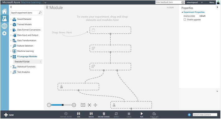
Figure 3-1. R Language modules in ML Studio
In this section, you will learn how to use the Execute R Script to perform sampling on a dataset. Follow these steps.
- From the toolbox, expand the Saved Datasets node, and click the Adult Census Income Binary Classification dataset. Drag and drop it onto the experiment design area.
- From the toolbox, expand the R Language Modules node, and click the Execute R Script module. Drag and drop it onto the experiment design area.
- Connect the dataset to the Execute R Script module. Figure 3-2 shows the experiment design.
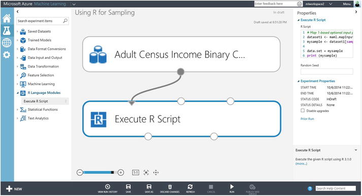
Figure 3-2. Using the Execute R Script to perform sampling on the Adult Census Income Binary Classification dataset
The Execute R Script module provides two input ports for datasets that can be used by the R script. In addition, it allows you to specify a Zip file that contains the R source script files that are used by the module. You can edit the R source script files on your local machine and test them. Then, you can compress the needed files into a Zip file and upload it to Azure Machine Learning through New > Dataset > From Local File path. After the Execute R Script module processes the data, the module provides two output ports: Result Dataset and an R Device. The Result Dataset corresponds to output from the R script that can be passed to the next module. The R Device output port provides you with an easy way to see the console output and graphics that are produced by the R interpreter.
Let’s continue creating your first R script using ML Studio.
- Click the Execute R Script module.
- On the Properties pane, write the following R script to perform sampling:
# Map 1-based optional input ports to variables
dataset1 <- maml.mapInputPort(1) # class: data.frame
mysample <- dataset1[sample(1:nrow(dataset1), 50, replace=FALSE),]

data.set = mysample
print (mysample)

# Select data.frame to be sent to the output Dataset port
maml.mapOutputPort("data.set");

R Script to perform sampling
To use the Execute R Script module, the following pattern is often used:
- Map the input ports to R variables or data frame.
- Main body of the R Script.
- Map the results to the output ports (see Figure 3-3).

Figure 3-3. Successful execution of the sampling experiment
To see this pattern in action, observe that in the R script provided, the maml.mapInputPort(1) method is used to map the dataset that was passed in from the first input port of the module to an R data frame. Next, see the R script that is used to perform sampling of the data. For debugging purposes, we also printed out the results of the sample. In the last step of the R script, the results are assigned to data.set and mapped to the output port using maml.mapOutputPort("data.set").
You are now ready to run the experiment. To do this, click the Run icon at the bottom pane of ML Studio. Figure 3-3 shows that the experiment has successfully completed execution.
Once the experiment has finished running, you can see the output of the R script. To do this, right-click on the Result Dataset of the Execute R Script module. Figure 3-4. shows the options available when you right-click on the Result Dataset of the Execute R Script module. Choose Visualize.
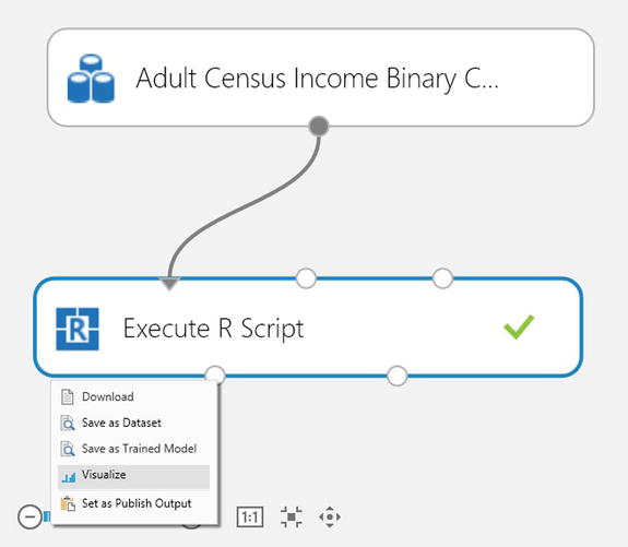
Figure 3-4. Visualizing the output of the R script
After you click Visualize, you will see that the sample consists of 50 rows. Each of the rows has 15 columns and the data distribution for the data. Figure 3-5 shows the visualization for the Result dataset.
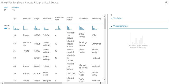
Figure 3-5. Visualization of result dataset produced by the R script
Congratulations, you have just successfully completed the integration of your first simple R script in Azure Machine Learning! In the next section, you will learn how to use Azure Machine Learning and R to create a machine learning model.
![]() Note Learn more about R and Machine Learning at http://ocw.mit.edu/courses/sloan-school-of-management/15-097-prediction-machine-learning-and-statistics-spring-2012/lecture-notes/MIT15_097S12_lec02.pdf.
Note Learn more about R and Machine Learning at http://ocw.mit.edu/courses/sloan-school-of-management/15-097-prediction-machine-learning-and-statistics-spring-2012/lecture-notes/MIT15_097S12_lec02.pdf.
Using R for Data Preprocessing
In many machine learning tasks, dimensionality reduction is an important step that is used to reduce the number of features for the machine learning algorithm. Principal component analysis (PCA) is a commonly used dimensionality reduction technique. PCA reduces the dimensionality of the dataset by finding a new set of variables (principal components) that are linear combinations of the original dataset, and are uncorrelated with all other variables. In this section, you will learn how to use R for preprocessing the data and reducing the dimensionality of dataset.
Let’s get started with using the Execute R Script module to perform principal component analysis of one of the sample datasets available in ML Studio. Follow these steps.
- Create a new experiment.
- From Saved Datasets, choose CRM Dataset Shared (see Figure 3-6).

Figure 3-6. Using the sample dataset, CRM Dataset Shared
- Right-click the output node, and choose Visualize. From the visualization shown in Figure 3-7, you will see that are 230 columns.

Figure 3-7. Initial 230 columns from the CRM Shared dataset
- Before you perform PCA, you need to make sure that the inputs to the Execute R Script module are numeric. For the sample dataset of CRM Dataset Shared, you know that the first 190 columns are numeric, and the remaining 40 columns are categorical. You first use the Project Columns, and set the Selected Column | column indices to be 1-190.
- Next, use the Missing Values Scrubber module to replace the missing value with 0, as follows:
- For missing values: Custom substitution value
- Replace with Value: 0
- Cols with all MV: KeepColumns
- MV indicator column: DoNotGenerate
- Once the missing values have been scrubbed, use the Metadata Editor module to change the data type for all the columns to be Integer.
- Next, drag and drop the Execute R Script module to the design surface and connect the modules, as shown in Figure 3-8.
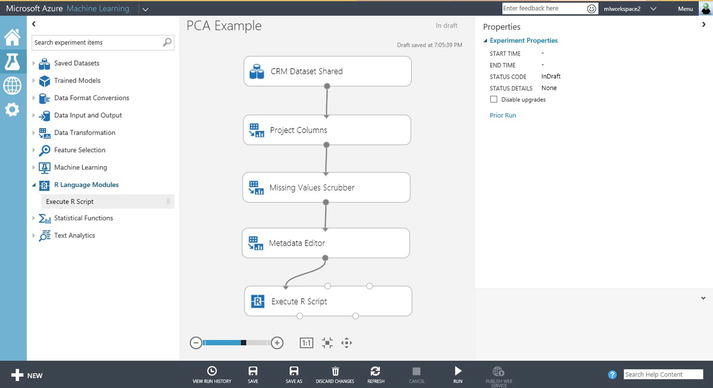
Figure 3-8. Using the Execute R Script module to perform PCA
- Click the Execute R Script module. You can provide the following script that will be used to perform PCA:
# Map 1-based optional input ports to variables
dataset1 <- maml.mapInputPort(1)
# Perform PCA on the first 190 columns
pca = prcomp(dataset1[,1:190])

# Return the top 10 principal components
top_pca_scores = data.frame(pca$x[,1:10])
data.set = top_pca_scores
plot(data.set)
# Select data.frame to be sent to the output Dataset port
maml.mapOutputPort("data.set");
Figure 3-9 shows how to use the script in ML Studio.

Figure 3-9. Performing PCA on the first 190 columns
- Click Run.
- Once the experiment has successfully executed, click the Result dataset node of the Execute R Script module. Click Visualize.
- Figure 3-10 shows the top ten principal components for the CRM Shared dataset. The principal components are used in the subsequent steps for building the classification model.
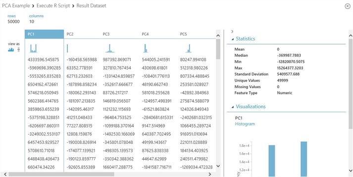
Figure 3-10. Principal components identified for the CRM Shared dataset
![]() Tip You can also provide a script bundle containing the R script in a Zip file, and use it in the Execute R Script module.
Tip You can also provide a script bundle containing the R script in a Zip file, and use it in the Execute R Script module.
If you have an R script that you have been using and want to use it as part of the experiment, you can Zip up the R script, and upload it to ML Studio as a dataset. To use a script bundle with the Execute R Script module, you will first need to package up the file in Zip format, so follow these steps.
- Navigate to the folder containing the R scripts that you intend to use in your experiment (see Figure 3-11).
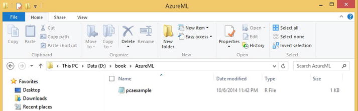
Figure 3-11. Folder containing the R script pcaexample.r
- Select all the files that you want to package up and right-click. In this example, right-click the file pcaexample.r, and choose Send to Compressed (zipped) folder, as shown in Figure 3-12.

Figure 3-12. Packaging the R scripts as a ZIP file
- Next, upload the zip file to ML Studio. TO do this, choose New DATASET
 From Local File. Select the Zip file that you want to upload, as shown in Figures 3-13 and 3-14.

Figure 3-13. New Dataset
From Local File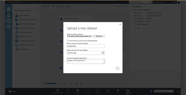
Figure 3-14. Uploading a new dataset
- Once the dataset has been uploaded, you can use it in your experiment. To do this, from Saved Datasets, select the uploaded Zip file, and drag and drop it to the experiment.
- Connect the uploaded Zip file to the Execute R Script module – Script Bundle (Zip) input, as shown in Figure 3-15.
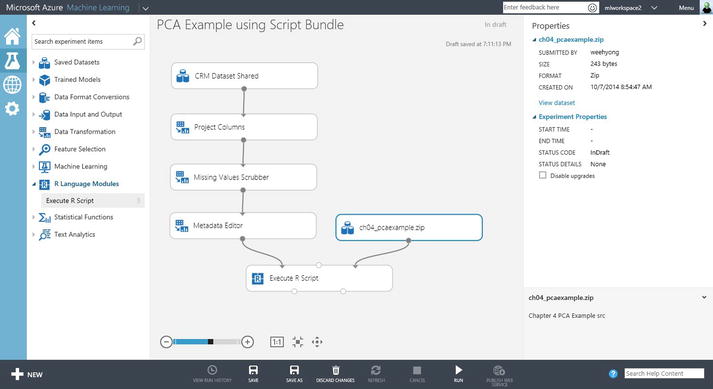
Figure 3-15. Using the script bundle as an input to the Execute R Script module
- In the Execute R Script module, specify where the R script can be found, as follows and as shown in Figure 3-16:
# Map 1-based optional input ports to variables
dataset1 <- maml.mapInputPort(1)
# Contents of optional Zip port are in ./src/
source("src/pcaexample.r");

# Select data.frame to be sent to the output Dataset port
maml.mapOutputPort("data.set");
Figure 3-16. Using the script bundle as inputs to the Execute R Script module
- You are now ready to run the experiment using the R script in the Zip file that you have uploaded to ML Studio. Using the script bundle allows you to easily reference an R script file that you can test outside of ML Studio. In order to update the script, you will have to re-upload the Zip file.
Building and Deploying a Decision Tree Using R
In this section, you will learn how to use R to build a machine learning model. When using R, you can tap into the large collection of R packages that implement various machine learning algorithms for classification, clustering, regression, K-Nearest Neighbor, market basket analysis, and much more.
![]() Note When you use the machine learning algorithms available in R and execute them using the Execute R module, you can only visualize the model and parameters. You cannot save the trained model and use it as input to other ML Studio modules.
Note When you use the machine learning algorithms available in R and execute them using the Execute R module, you can only visualize the model and parameters. You cannot save the trained model and use it as input to other ML Studio modules.
Using ML studio, several R machine learning algorithms are provided. For example, you can use the R Auto-ARIMA module to build an optimal autoregressive moving average model for a univariate time series. You can also use the R K-Nearest Neighbor Classification module to create a k-nearest neighbor (KNN) classification model.
In this section, you will learn how to use an R package called rpart to build a decision tree. The rpart package provides you with recursive partitioning algorithms for performing classification and regression.
![]() Note Learn more about the rpart R package at http://cran.r-project.org/web/packages/rpart/rpart.pdf.
Note Learn more about the rpart R package at http://cran.r-project.org/web/packages/rpart/rpart.pdf.
For this exercise, you will use the Adult Census Income Binary Classification dataset. Let’s get started.
- From the toolbox, drag and drop the following modules on the experiment design area:
- Adult Census Income Binary Classification dataset (available under Saved Datasets)
- Project Columns (available from Data Transformation Manipulation)
- Execute R Script module (found under R Language modules)
- Connect the Adult Census Income Binary Classification dataset to Project Columns.
- Click Project Columns to select the columns that will be used in the experiment. Select the following columns: age, sex, education, income, marital-status, occupation.
Figure 3-17 shows the selection of the columns and Figure 3-18 shows the completed experiment and the Project Columns properties.

Figure 3-17. Selecting columns that will be used

Figure 3-18. Complete Experiment
- Connect the Project Columns to Execute R Script.
- Click Execute R Script and provide the following script. Figure 3-19 shows the R script in ML studio.
library(rpart)

# Map 1-based optional input ports to variables
Dataset1 <- maml.mapInputPort(1) # class: data.frame

fit <- rpart(income ~ age + sex + education + occupation,method="class", data=Dataset1)

# display the results, and summary of the splits
printcp(fit)
plotcp(fit)
summary(fit)

# plot the decision tree
plot(fit, uniform=TRUE, margin = 0.1,compress = TRUE, main="Classification Tree for Census Dataset")
text(fit, use.n=TRUE, all=TRUE, cex=0.8, pretty=1)

data.set = Dataset1

# Select data.frame to be sent to the output Dataset port
maml.mapOutputPort("data.set");

Figure 3-19. Experiment for performing classification using R script
In the R script, first load the rpart library using library(). Next, map the dataset that is passed to the Execute R Script module to a data frame.
To build the decision tree, you will use the rpart function. Several type of methods are supported by rpart: class (classification), and anova (regression). In this exercise, you will use rpart to perform classification (i.e. method="class"), as follows:
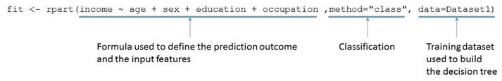
The formula specified uses the format: predictionVariable ~ inputfeature1 + inputfeature2 + ...
After the decision tree has been constructed, the R script invokes the printcp(), plotcp(), and summary() functions to display the results, and a summary of each of the split values in the tree. In the R script, the plot() function is used to plot the rpart model. By default, when the rpart model is plotted, an abbreviated representation is used to denote the split value. In the R script, the setting of pretty=1 is added to enable the actual split values to be shown (see Figure 3-20).

Figure 3-20. The R script in ML Studio
You are now ready to run the experiment. To do this, click the Run icon at the bottom pane of ML Studio. Once the experiment has executed successfully, you can view the details of the decision tree and also visualize the overall shape of the decision tree.
To view the details of the decision tree, click the Execute R Script module and View output log (shown in Figure 3-21) in the Properties pane.
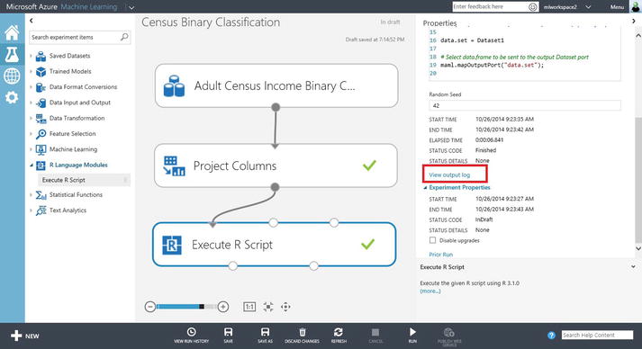
Figure 3-21. View output log for Execute R Script
A sample of the output log is shown:
[ModuleOutput] Classification tree:
[ModuleOutput]
[ModuleOutput]
[ModuleOutput]
[ModuleOutput] Variables actually used in tree construction:
[ModuleOutput]
[ModuleOutput] [1] age        education  occupation sex
[ModuleOutput]
[ModuleOutput]
...
[ModuleOutput]   Primary splits:
[ModuleOutput]
[ModuleOutput]       education  splits as  LLLLLLLLLRRLRLRL, improve=1274.3680, (0 missing)
[ModuleOutput]
[ModuleOutput]       occupation splits as  LLLRLLLLLRRLLL, improve=1065.9400, (1843 missing)
[ModuleOutput]
[ModuleOutput]       age        < 29.5 to the left,  improve= 980.1513, (0 missing)
[ModuleOutput]
[ModuleOutput]       sex        splits as  LR, improve= 555.3667, (0 missing)
To visualize the decision tree, click the R Device output port (i.e. the second output of the Execute R Script module), and you will see the decision tree that you just constructed using rpart (shown in Figure 3-22).

Figure 3-22. Decision tree constructed using rpart
![]() Note Azure Machine Learning provides a good collection of saved datasets that can be used in your experiments. In addition, you can also find an extensive collection of datasets at the UCI Machine Learning Repository at http://archive.ics.uci.edu/ml/datasets.html.
Note Azure Machine Learning provides a good collection of saved datasets that can be used in your experiments. In addition, you can also find an extensive collection of datasets at the UCI Machine Learning Repository at http://archive.ics.uci.edu/ml/datasets.html.
Summary
In this chapter, you learned about the exciting possibilities offered by R integration with Azure Machine Learning. You learned how to use the different R Language Modules in ML Studio. As you designed your experiment using R, you learned how to map the inputs and outputs of the module to R variables and data frames. Next, you learned how to build your first R script to perform data sampling and how to visualize the results using the built-in data visualization tools available in ML Studio. With that as foundation, you moved on to building and deploying experiments that use R for data preprocessing through an R Script bundle and building decision trees.