![]()
Query Strategies
In the previous chapter, you looked at strategies to identify potential indexes for your databases. That, though, is often only half the story. Once the indexes have been created, you would expect performance within the database to improve, leading you then to the next bottleneck. Unfortunately, coding practices and selectivity can sometimes negatively influence the application of indexes to queries. And sometimes how the database and tables are being accessed will prevent the use of some of the most beneficial indexes in your databases.
This chapter covers a number of querying strategies where indexes may not be used as you may have expected. These scenarios are
- LIKE comparison
- Concatenation
- Computed columns
- Scalar functions
- Data conversions
In each scenario, you’ll look at the circumstances around them and why they don't work as expected. Then you’ll see some ways to mitigate the issues and some tips on how to use the right index in the right place. By the end of the chapter, you’ll be more prepared to recognize situations that will hamper your ability to index the database for performance, and you’ll have the tools to begin mitigating these risks.
When looking at the impact of queries on the use of indexes, the first place to start is with the LIKE comparison. The LIKE comparison allows searches in columns on any single character or pattern. If you need to find all the values in a table that start with the letters AAA or BBB, the LIKE comparison provides this functionality. In these searches, the query can read through the index and find the values that match to the characters or pattern, since the index is sorted. Problems can arise when using this comparison in queries to find values that contain or end with a character or pattern.
In this situation, the sort of the index becomes immaterial because statistics are collected only on the left edge of character values. The likelihood that the letter B appears in the first value in the index is equal to it appearing in the last value in the index. To determine which records in the table have a B in the column, all rows must be checked. There are no statistics available to identify the expected likelihood of occurrences. Without reliable statistics to use, SQL Server will not know what index to use to satisfy a query and may end up using a poor execution plan.
To understand the problems that can occur with the LIKE comparison, you’ll walk through a few demonstrations that show both scenarios and their related statistics. Let’s start with querying the Person.Address table for records where AddressLine1 starts with 710 (see Listing 12-1). A review of the STATISTICS IO output in Figure 12-1 shows the query required three logical reads. Examining the execution plan in Figure 12-2 shows an index seek on the nonclustered index, which results in three logical reads.

Figure 12-1. STATISTICS IO for addresses beginning with 710

Figure 12-2. Execution plan for addresses beginning with 710
In this situation, the LIKE comparison worked well and the execution plan, statistics, and I/O were all appropriate for the request. Unfortunately, as mentioned, this isn’t the only manner in which LIKE comparisons can be used. The comparison can be used to find values within a column. Consider a scenario where you need to find all the addresses that match a specific street name of a road, such as Longbrook (see Listing 12-2). With this query, the execution plan uses a scan on the nonclustered index and requires 216 logical reads, as shown in Figure 12-3. Figure 12-4 shows the execution plan.

Figure 12-3. STATISTICS IO for addresses containing “Longbrook”

Figure 12-4. Execution plan for addresses containing “Longbrook”
In this scenario, the table and index were both small. The difference between an index seek and an index scan was not too extreme. Consider if this scenario was happening in your production system with one of the larger tables in your databases. Instead of being able to quickly filter out records that match the search values, SQL Server is required to look through all rows, which could potentially lead to blocking and deadlocking issues.
A popular method of avoiding this situation is to declare that wildcards are never allowed on the left edge of searches. Unfortunately, this is a fairly unrealistic expectation. There are few business managers in the world that would agree to require their users to enter all possible street number combinations in an attempt to find every address that matched the street name search. Just reading it here sounds silly.
A less popular but much more appropriate and useful solution to this scenario is to create a full-text index on the table. A contributing factor to full-text indexes being less popular than nonclustered indexes is because of the difference in building and creating them, which has made them less familiar to most people. With a full-text index, words within one or more columns are cataloged, along with their position in the table. This enables the query to search quickly for the discrete values within a column value without having to check all the records in an index.
To use a full-text index on the Person.Address table, you must first build a full-text catalog, as shown in Listing 12-3. After that, the full-text index is created and includes the column that will be searched in the queries. Lastly, the query needs to be modified to use one of the full-text predicate functions. In this example, you will be using the CONTAINS function.
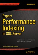
With the full-text index in place, the performance of the search for streets named Longbrook is similar to the first search where the query was looking for addresses starting with 710. In the execution plan in Figure 12-6, instead of a scan of the nonclustered index, the query is using a seek operation on the clustered index with a table-valued function lookup against the full-text index. As a result, instead of the 216 logical reads when using the LIKE comparison, using the full-text index requires only 12 logical reads (shown in Figure 12-5). The difference in reads provides a substantial improvement in performance over the first search attempt.

Figure 12-5. STATISTICS IO for addresses using CONTAINS
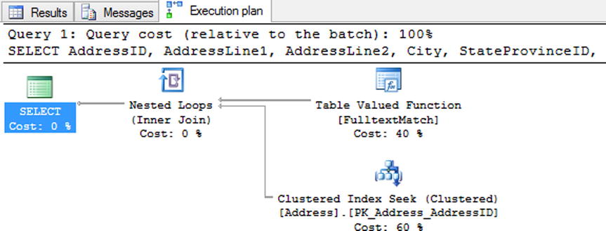
Figure 12-6. Execution plan for addresses using CONTAINS
For more information on full-text indexes, read Chapter 6.
Another scenario that can wreak havoc on indexing strategies is the use of concatenation. Concatenation is when two or more values are appended to one another. When this happens in a WHERE clause, it can often lead to poor performance that wasn’t expected.
To demonstrate this scenario, consider a query for someone with the name Gustavo Achong. Searching for this value requires using the FirstName and LastName columns, which are concatenated together with a space between the columns. Listing 12-4 shows the query. A script to build and index on these columns is also included in the code listing. The execution plan generated for this query, shown in Figure 12-8, shows that the new index is used but that the index is being scanned instead of a seek operation being used. Even though the leading left edge of the index matches the left side values of the concatenated values, the index is not able to determine where in the index to find the values. This results in the index using 99 logical reads to return the query results, shown in Figure 12-7.
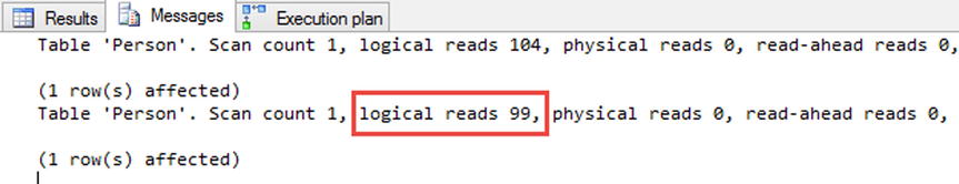
Figure 12-7. STATISTICS IO for concatentation

Figure 12-8. Execution plan for concatentation
As mentioned, using a scan on the index is not necessarily a bad thing. However, using a scan when there are a lot of concurrent users or data modifications occurring could lead to a performance issue. When it comes to larger tables with millions or more records, this can possibly lead to a lack of scalability for the database.
You might think that removing the space between the first and last names is a good idea (see Listing 12-5). The major issue with this solution is that it doesn’t work. As the execution plan in Figure 12-10 shows, it’s nearly identical to the one with the space in the concatenated value with the same 99 reads as well (shown in Figure 12-9).
Figure 12-9. STATISTICS IO for concatenation without spaces

Figure 12-10. Execution plan for concatenation without spaces
Probably the best way to fix issues with concatenated values is to remove the need to concatenate. Instead of searching for the value Gustavo Achong, instead search for the first name Gustavo and the last name Achong (see Listing 12-6). When this change is made, the query is then able to use a seek operation on the nonclustered index and return the results with only two logical reads (see Figure 12-11). These results are a definite improvement over when the values were concatenated together. See Figure 12-12 for the execution plan.

Figure 12-11. STATISTICS IO for concatenation removed

Figure 12-12. Execution plan with concatenation removed
At times, you won’t have the option to remove concatenation from a query. In these cases, there is another way to resolve index performance issues: the concatenated values can be added to the table as a computed column. This solution, along with some of its issues, is discussed in the next section.
Computed Columns
Sometimes one or more columns in a table are defined as an expression. These types of columns are referred to as computed columns. Computed columns can be useful when you need a column to hold the result of a function or calculation that will change over time based on the other columns in the table. Rather than spending the people cycles to make certain that all modifications to a table always include changes to all the related columns, the components can be changed and the results computed afterward.
Note that computed columns cannot leverage the indexes on the source columns for the computed column. To demonstrate, add two computed columns to the Person.Person table using Listing 12-7. The first column will concatenate FirstName and LastName together, as they were concatenated in the previous section. The second column will multiply ContactID by EmailPromotion; this calculation doesn’t mean anything, but it will show how this can be used with other calculation types.
With the columns in place, the next step is to execute a couple of queries against the table. Execute two queries against the table using Listing 12-8. The first query is similar to the first and last name query from the previous section (when searching for Gustavo Achong). The second query will return all records with the CalculatedValue of 198.
After executing both queries, the execution plans in Figure 12-14 show that both used scan operations to return the query results. These results are less than ideal for the same reasons mentioned earlier in this chapter: in some situations they can lead to blocking and utilize more I/O than should be necessary for the query request. By more I/O, the query results for both require read I/Os from scanning the entire table, shown in Figure 12-13.

Figure 12-13. STATISTICS IO for computed columns

Figure 12-14. Computed column execution plans
An indexing option available for computed columns is to index the computed columns themselves. As the query for FirstLastName shows, the query can use any of the indexes on the table. The restriction is that they can’t use them any better than if the expression for the computed column was in the query itself. Indexing the computed columns, as shown in Listing 12-9, provides the necessary distribution and record information to allow queries, such as those in Listing 12-8, to use seeks instead of scans. The index materializes the values in the computed column, allowing quick access to the data, which results in a significant reduction in I/O from 99 to 5 reads and 3.878 to 2 reads, shown in Figure 12-15. Figure 12-16 shows the execution plan.

Figure 12-15. STATISTICS IO for indexed computed column

Figure 12-16. Indexed computed column execution plans
![]() Note When indexing a computed column, the expression for the column must be deterministic. This means that every time the expression executes with the same variables, it will always return the same results. As an example, using GETDATE() in a computed column expression would not be deterministic.
Note When indexing a computed column, the expression for the column must be deterministic. This means that every time the expression executes with the same variables, it will always return the same results. As an example, using GETDATE() in a computed column expression would not be deterministic.
As this section demonstrates, computed columns can be extremely useful when expressions are needed to define values as part of a table. For instance, if an application can only send in searches where the first and last names were combined, computed columns can provide the data in the format that the application is sending. The columns can use underlying indexes to return results but can’t use the statistics for those indexes because of the expression in the column definition. To index these types of columns, the computed column itself must be indexed.
Scalar Functions
The previous few sections discussed filtering query results by searching within column values or by combining values across columns. This section looks at the effect of scalar functions used in the WHERE clauses of queries. Scalar functions provide the ability to transform values to other values that can be more useful than the original value when querying the database.
User-defined scalar functions can also be created and used in the WHERE clause. The trouble with both system and user-defined scalar functions is that they change the values in the index to something other than what was indexed by SQL Server. Because the values of the calculations are not known until runtime, the query optimizer does not have statistics to determine the frequency of values in the index or information on where the calculated values are located in the index or table.
To demonstrate the effect of scalar functions on queries, consider the two queries in Listing 12-10 that return information from Person.Person. Both queries will return all rows that have the value Gustavo in the FirstName column. The difference between the two queries is that the second query will use the RTRIM function in the WHERE clause on the FirstName column.
As the execution plan in Figure 12-18 shows, when the scalar function is added to the WHERE clause, the execution plan utilizes an index scan instead of an index seek. This change increases the I/Os from 2 to 99 (shown in Figure 12-17), which is similar to other examples. In this example, just excluding the scalar function, as in the first query, can provide the same results as with the function in place. That won’t be the case for all queries, but the way to allow indexes to be best used is to move the scalar function from the key columns to the parameters of a query.

Figure 12-17. Execution plans for Gustavo queries

Figure 12-18. Execution plans for Gustavo queries
A good example of how scalar functions can be moved off of key columns and into the parameters is when the functions MONTH and YEAR are used. Suppose a query needs to return all the sales orders for the year 2001 and for December. This could be accomplished with the first SELECT query in Listing 12-11. Unfortunately, using the MONTH and YEAR functions change the value of OrderDate, and the index that was built cannot be used (see the first execution plan in Figure 12-20). This issue can be avoided by changing the query in such a way that, instead of using the functions, you filter against a range of values, such as in the second SELECT statement in Listing 12-11. As the second execution shows, the query is able to return the results with a seek instead of a scan, providing a significant reduction in reads, from 73 to 3, as shown in Figure 12-19.

Figure 12-19. Execution plans for date queries

Figure 12-20. Execution plans for date queries
It won’t always be possible to remove scalar functions from the WHERE clause of queries. One good example of this is if leading spaces were added to a column that should not be included when comparing the column values to parameters. In such a situation, you will need to think a little more “outside the box.” One possible solution is to use a computed column with an index on it, as suggested in the previous section.
The important thing to remember when dealing with scalar functions in the WHERE clause is that if the function changes the value of a column, any index on the column most likely won’t be able to be used for the query. If the table is small and the queries will be infrequent, this may not be a significant problem. For larger systems, this may be the reason behind unexpected high numbers of scans on indexes.
One last area where queries can negatively affect how indexes are used is when the data types of columns change within a JOIN operation or WHERE clause. When data types don’t match in either of those conditions, SQL Server needs to convert the values in the columns to the same data types. If the data conversion is not included in the syntax of the query, SQL Server will attempt the data conversion behind the scenes.
The reason that data conversions can have a negative effect on query performance is along the same lines as the issues related to scalar functions. If a column in an index needs to be changed from varchar to int, the statistics and other information for this index won’t be useful in determining the frequency and location of values. For instance, the number 10 and the string "10" would likely be sorted into entirely different positions in the same index. To illustrate the effect that data conversions can have on a query, start by executing the code in Listing 12-12.
Listing 12-12 will create a table with varchar data in it. It will then add two indexes to the table that will be used in the demonstration queries. The two sample queries, shown in Listing 12-13, will be used to show how data conversions can affect the performance and utilization of an index. For both queries, the RECOMPILE option is being utilized to prevent bad parameter sniffing, which occurs when the option is not being used.
![]() Note For more information on parameter sniffing, read Paul White’s “Parameter Sniffing, Embedding, and the RECOMPILE Options” article on SQLPerformance.com at http://sqlperformance.com/2013/08/t-sql-queries/parameter-sniffing-embedding-and-the-recompile-options.
Note For more information on parameter sniffing, read Paul White’s “Parameter Sniffing, Embedding, and the RECOMPILE Options” article on SQLPerformance.com at http://sqlperformance.com/2013/08/t-sql-queries/parameter-sniffing-embedding-and-the-recompile-options.
The first SELECT query uses the @FirstName variable with the nvarchar data type. This data type does not match the data type for the column in the table PersonContact, so the column in the table must be converted from varchar to nvarchar. The execution plan for the query (Figure 12-21) shows that the query is using an index seek on the nonclustered index to satisfy the query, and the predicate is converting the data in the column to nvarchar, with a key lookup on the clustered index for the columns not in the nonclustered index. Also note that the cost for the first query is 40 percent of the total batch, which is just the two queries.
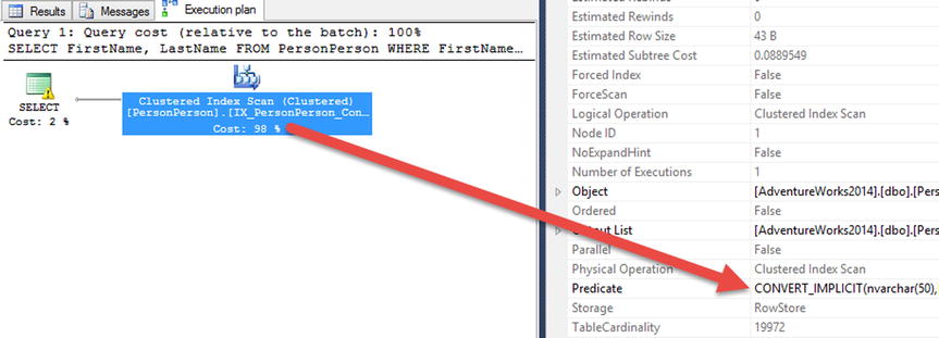
Figure 12-21. Execution plans with implicit data conversion
![]() Note The additional information shown for the operators in the execution plans is available in the Properties window in SQL Server Management Studio. The Properties windows is full of useful information about the operations from the columns that are used for estimated and actual row counts.
Note The additional information shown for the operators in the execution plans is available in the Properties window in SQL Server Management Studio. The Properties windows is full of useful information about the operations from the columns that are used for estimated and actual row counts.
One other item to note in the execution plan in Figure 12-22 is the warning included on the SELECT operation for the first query. With the release of SQL Server 2012 there are now new warning messages included in execution plans that contain implicit conversions. The warning message appears as a yellow triangle with an exclamation point in it. Hovering over the operator will display properties of the operator and the warning message. These messages include information detailing what column is being converted and the issue associated with the problem. In this case, the issue is CardinalityEstimate. In other words, SQL Server doesn’t have statistics necessary to build an execution plan that knows the frequency of the values in the predicate.

Figure 12-22. Warning included with implicit conversion
The second SELECT query in Listing 12-13 uses a variable with a varchar data type. Since this data type already matches the data type of the column in the table, the nonclustered index can be used. As the execution plan in Figure 12-23 shows, with matching data types the query optimizer can build a plan that knows where the rows in the index are and can perform a seek to obtain them.

Figure 12-23. Execution plans without data conversion
Interestingly enough, the cost of the second plan is 60 percent of the batch, which should mean that the second plan performed more poorly than the first. This isn’t the case, though, as you can see if you review the logical reads from STATISTICS IO, shown in Figure 12-24. For the first query, the number of reads was 89 logical reads. The second query had only 18 reads. The difference in the reads is because of the cardinality estimation issue. The execution plan didn’t know the frequency from statistics in which the name being queried would appear in the index. It estimated that there would be far fewer rows than there were, so it built a plan with an index seek and key lookup to return the rows. The operations required to satisfy that plan resulted in more than twice the number of reads than if the entire table was scanned for the value.

Figure 12-24. STATISTICS IO for implicit conversion queries
In this section, the discussion mostly focused on implicit data conversions. While these can be more silent that explicit data conversions, the same concepts and mitigations apply to these data conversions. Since they are more intentional, they should be less frequent. Even so, when performing data conversions, pay close attention to the data types because how they are changed will impact query performance and index utilization.
Summary
In this chapter, you examined the effect that queries can have on whether indexes can provide the expected performance improvements. There are times when a specific type of index may not be appropriate for a situation, such as searching for values within character values in large tables. In other situations, applying the right type of index or function in the right place can have a significant impact on whether the query can utilize an index.
In many of the examples in this chapter, the offending usage of an index was when it utilized a scan on the index instead of a seek operation. For these scenarios, index seeks were the ideal index operation. This won’t always be the case and there are situations where scans against an index are significantly more ideal than seek operations. It’s important to remember what type of transactions the environment is geared for and the size of the tables that are being accessed.
The main take-away from this chapter is that you should take care when writing queries. The choices made when developing database code can completely unravel the work done to properly index a database. Be sure to complement your indexes with code that leverages them to their max.