![]()
Indexing Strategies
Indexing databases is often thought of as an art where the database is the canvas and the indexes are the paints that come together to form a beautiful tapestry of storage and performance. A little color here, a little color there, and paintings will take shape. In much the same way, a clustered index on a table and then a few nonclustered indexes can result in screaming performance as beautiful as any masterpiece. Going a little too abstract or minimalist with your indexing might make you feel good, but the performance will let you know it isn’t too useful.
As colorful as this analogy is, there is more science behind designing and applying indexes than there is artistry. A few columns pulled together because they might work well together is often less beneficial than an index built upon well-established patterns. The indexes that are based on tried-and-true practices are often the best solutions. In this chapter, you’ll walk through a number of patterns to help identify potential indexes.
Heaps
There are few valid cases for using heaps in your databases. The general rule of thumb for most DBAs is that all tables in database should be built with clustered indexes instead of heaps. While this practice rings true in many situations, there are situations when using a heap is acceptable and preferred. This section looks at one of these scenarios and discusses the other situations in generalities. The reason for being generic is that it is difficult to make blanket statements about when to use a heap instead of a clustered index (which will be explained more later in the section).
One of the situations in which heaps are useful is with temporary objects, such as temporary tables and table variables. When we use these objects, we often create them without thinking or considering building a clustered index on them. The result is that we use more heaps on tables than we think we do.
Consider for a moment the last time you created a table variable or a temporary table. Did the syntax for the object specifically create a CLUSTERED index or a PRIMARY KEY with the default configuration? If not, then the temporary object was created as a heap. This isn’t necessarily a travesty. It is common in most workloads—not necessarily a call to arms to change your coding practices. As I’ll demonstrate in the examples in this section, the performance between a temporary object with a heap or a clustered index can be immaterial.
For this example, let’s start with a simple use case for a temporary table. The example uses the table Sales.SalesOrderHeader from which you’ll retrieve a few rows based on a SalesPersonID and then insert them into a temporary table. The temporary table will be used to return all rows from Sales.SalesOrderDetail that match the results in the temporary table. Two versions of the example will be used to demonstrate how using a heap or a clustered index on the temporary table doesn’t change the query execution.
In the first version of the example, shown in Listing 11-1, the temporary table is built using a heap. This is the method that people often use to create temporary objects. As the execution plan in Figure 11-1 shows, when the temporary table is accessed, identified by the arrow, a table scan is used to access the rows in the object. This behavior is expected with a heap. Since the rows aren’t ordered, there is no way to access specific rows without checking all the rows first. To find all the rows in Sales.SalesOrderDetail that match those in the temporary table, the execution plan uses a nested loop with an index seek.

Figure 11-1. Execution plan for heap temporary object
In the second version of the script, shown in Listing 11-2, the temporary table is created instead with a clustered index on the SalesOrderID column. The index is the only difference between the two scripts. This difference results in a slight change in the execution plans. Figure 11-2 shows the clustered index version of the execution plan. The difference between the two plans is that instead of a table scan, there is a clustered index scan against the temporary table. While these are different operations, the work done by both is essentially the same. During query execution, all rows in the temporary object are accessed while joining them to rows in Sales.SalesOrderDetail.

Figure 11-2. Execution plan for clustered temporary object
![]() Note With SQL Server 2014, table variables can have both clustered and nonclustered indexes on them. The requirement is that the indexes are created when the variable is declared. DDL operations are not allowed on table variables after they are defined.
Note With SQL Server 2014, table variables can have both clustered and nonclustered indexes on them. The requirement is that the indexes are created when the variable is declared. DDL operations are not allowed on table variables after they are defined.
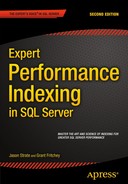
In queries similar to the example in this section, the execution plans for temporary tables with heaps and clustered indexes are nearly the same. As with all rules, there may be exceptions where performance will differ. A good example of when using a heap can affect performance is the T-SQL syntax that leverages a sort in its execution. Listing 11-3 shows a specific example using EXISTS in the WHERE clause. Figure 11-3 shows the execution plan for the query. Before the nested loop joins to resolve the EXISTS predicate, the data must first be sorted. In this case, the use of a heap has hindered the performance of the query because the heap table forces a sort operation. With small datasets, the performance difference may not be noticeable. As the size of dataset increases, little changes such as the inclusion of a sort operation can compound the performance of your queries.
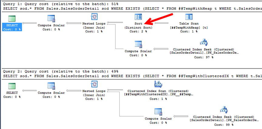
Figure 11-3. EXISTS example execution plan
Generally, the other scenarios where using heaps makes sense are few and far between. The reason using temporary objects makes sense is because of the low frequency in which the data will be accessed compared to the amount of time it will take to create a structure, such as a clustered index, to support the performance. This scenario can also carry over the staging tables, since the data is usually inserted and modified a couple times before moving it to its final destination.
In high-insert environments, it might seem to make sense to use heaps to avoid the overhead of maintaining the B-tree. The trouble with this scenario is that the gains on inserts are offset by the need to access the data, which requires other nonclustered indexes, which then have sort orders to maintain.
When confronted with a situation for using heaps on your tables, first look at whether clustered indexes can be proven to be a burden on the storage of the data before using them. And before looking to the heap, also consider whether newer indexing structures such as clustered columnstore indexes or memory-optimized tables provide the performance required.
The main point of this section is that heaps are used quite often in the real world. While most practices rail against their use, there are some cases and situations where they are a good fit. As the discussion moves into clustered indexes, you will see why it is usually a good idea to default to clustered indexes and use heaps in the situations where either it won’t matter, such as temporary objects, or they outperform clustered indexes.
Throughout this book, the value of and preference for using a clustered index as the structure for organizing the data page of a table has been discussed. Clustered indexes organize the data in their tables based on the key columns for the clustered index. All the data pages for the index are stored logically according to the key columns. The benefit of this is optimal access to the data through the key columns.
New tables should nearly always be built with clustered indexes. The question, though, when building the tables is what should be selected for the key columns in the clustered index. There are a few characteristics that most often are attributed to well-defined clustered indexes. These characteristics are
- Static
- Narrow
- Unique
- Ever-increasing
There are a number of reasons that each of these attributes help create a well-defined clustered index.
First, a clustered index should be static. The key columns defined for the clustered index should be expected to be static for the lifetime of the row. By using a static value, the position of the row in the index will not change when the row is updated. When nonstatic key columns are used, the position of the row in the clustered index can change, which would require the row to be inserted on a different page. Also, nonclustered indexes would need to be modified to change the key columns’ values stored in those indexes. All of this together leads to the potential for fragmentation of the clustered and nonclustered indexes on a table.
The next attribute that a clustered index should have is that it is narrow. Ideally, there should be only a single column for the clustered index key. These columns should be defined with the smallest data type reasonable for that data being stored in the table. Narrow clustered indexes are important because the clustered index key for every row is included in all nonclustered indexes associated with the table. The wider the clustered index key, the wider all nonclustered indexes will be, and the more pages they will require. As discussed in other sections, the more pages in an index, the more resources are required to use the index. This can affect the performance of queries.
Clustered indexes should also be unique. Clustered indexes store a single row in a single location in the index; for duplicate rows within the key columns of a clustered index, the uniquifier provides the uniqueness required for the row. When the uniquifier is added to a row, it is extended by 4 bytes, which changes how narrow the clustered index is and results in the same concerns that are associated with a non-narrow clustered index. You can find more information on the uniquifier in Chapter 2.
Lastly, a well-defined clustered index will be based on an ever-increasing value. Using an ever-increasing clustered key causes new rows to be added to the end of the clustered index. Placing new rows at the end of the B-tree reduces the fragmentation that would likely occur if the row were inserted in the middle of the clustered index.
One additional consideration when selecting the clustered index key columns is that they represent the columns in the row that will most frequently be used to access the row. Are there specific columns or values that will most often be used to retrieve rows from the table? If so, these columns are good candidates for the clustering index key. In the end, queries against the table will perform best when they can access data through the path of least resistance.
While considering the previous guidelines for selecting clustered index strategies, there are a number of patterns that can be used to identify and model clustered indexes. The clustered index patterns are
- Identity/Sequence
- Surrogate Key
- Foreign Key
- Multiple Column
- Globally Unique Identifier
In the rest of this section, I’ll walk you through each of the patterns, describing each and how to identify when to utilize the pattern.
The most frequent pattern of building a clustered index is to pair it with a column on a table that has been configured to be ever-increasing using either the IDENTITY property or the SEQUENCE object. In this pattern, the IDENTITY column is often also the PRIMARY KEY on the table. The data type is often an integer, which includes tinyint, smallint, int, and bigint. The primary benefit of this pattern is that it achieves all the attributes of a well-defined clustered index. It is static, narrow, unique, and ever-increasing. When you consider how the data in the table will be accessed, in most cases the key value will most often be used to access rows in the table.
One distinction of the Identity Sequence pattern is that the column used for the clustered index key has no relationship between the data in the row and the clustered index key. To implement the pattern, a new column is added to the table that contains the IDENTITY property or SEQUENCE default. This column is then set as the clustered index key and often the PRIMARY KEY as well.
Examples of this pattern can be found in nearly all databases. Creating a table with this pattern would look similar to the CREATE TABLE statements in Listing 11-4. Both tables are built to contain fruit: two apple rows, a banana row, and grape row are inserted. The Color column would not have been a good clustering key since it does not identify the rows in the table. The FruitName column could have identified the rows in the table, except it isn’t unique across the table, which would have required the uniquifier and led to a larger clustering key. Indexing the table to the Identity Sequence pattern, a FruitID column is created.
One of the effects of using the Identity Sequence pattern is that the value for the clustering key column has no relationship to the information that it represents. In the query output from Listing 11-1, which is shown in Figure 11-4, the value of 1 is assigned to the first row inserted for both result sets. Then, a value of 2 is assigned for the next row, and so on. As more rows are added, the FruitID column increments and doesn’t require any single piece of information in the record in order to designate the instance of information.

Figure 11-4. Results for Identity Sequence pattern
![]() Note SEQUENCE was a new object in SQL Server 2012. Through sequences, ranges of numeric values can be generated, which are either ascending or descending. A sequence is not associated with any specific table. If you are unfamiliar with using SEQUENCE, it is recommended that you consider using sequences over IDENTITY for performance and control purposes. They are outside the context of this book.
Note SEQUENCE was a new object in SQL Server 2012. Through sequences, ranges of numeric values can be generated, which are either ascending or descending. A sequence is not associated with any specific table. If you are unfamiliar with using SEQUENCE, it is recommended that you consider using sequences over IDENTITY for performance and control purposes. They are outside the context of this book.
In some cases, using a surrogate key in the data for the clustering key is as valid as adding an identity column to the table to use for the Identity Sequence pattern. A surrogate key is a column in the data that can uniquely identify one row from all the other rows. The cases where using a surrogate key is valid can be identified when there is a surrogate key in the data that meets the attributes of a well-defined clustering key. When using surrogate keys for clustering keys, they are not likely to be ever-increasing, but they should still be unique, narrow, and static.
A common example of when a surrogate key may be used instead of an identity column is when looking at tables that contain one- or two-character abbreviations for the information they represent. These abbreviations may be for the status of an order, the size of a product, or a list of states or provinces. Compared to using an int, which is 4 bytes, in the Identity Column pattern, using a char(1) or char(2) data type with the Surrogate Key pattern will result in a clustering key that is more narrow than the former.
The Surrogate Key pattern also provides the additional benefit of providing an easier-to-decipher key value. When using the Identity Sequence pattern, there is no inherent meaning when the clustering key has a value of 1 or 7. These values are meaningless—intentionally so. With the Surrogate Key pattern, the abbreviations of O and C represent real information (Opened and Closed, respectively).
As a simple example of the Surrogate Key pattern, let’s consider a table that contains states and their abbreviations. You’ll also include the name of the country for the states. Listing 11-5 shows the SQL to create and populate the table. The table has a StateAbbreviation column, which is a char(2). Since this is a narrow, unique, and static value for each state, the clustered index is created on the column. Next, a few rows are added to the table for the four states that the fictitious database requires.
In situations where the surrogate key matches the Surrogate Key pattern, the technique in Listing 11-5 can be a useful way of selecting the clustering key column. Reviewing the contents of dbo.IndexStrategiesSurrogate (shown in Figure 11-5), the four rows are in the table, and using StateAbbreviation in another table as a foreign key value can be useful since the value MN has some inherent meaning.

Figure 11-5. Results for Surrogate Key pattern
This pattern may seem ideal and more worthwhile than the Identity Column pattern—especially since the value of the clustering key helps describe the data. However, there are a few downsides to using this pattern, which relate to the attributes that can make it a well-defined clustering key.
First, let’s consider the uniqueness of the clustering key. Provided that the use cases for the database and table never change, there can be trust that the values will remain unique. What happens, though, when the database needs to be used in an international context? If states for other countries such as the Netherlands need to be included, there is a great potential for data issues. In the Netherlands, FL is the abbreviation for Flevopolder, and NH is the abbreviation for Noord-Holland. Sending an order to Florida that should go to Flevopolder can have serious business consequences. To retain the uniqueness, something outside of the two-character abbreviation would need to be added to the surrogate key and clustering key.
Changing the surrogate would then affect the narrowness of the clustering key. There are probably two approaches that could be taken to address this problem. The first option is to add another column to the surrogate key to identify whether a state abbreviation belongs to one country or another. The other option is to increase the size of the state abbreviation to include a country abbreviation in the same column. With either of the solutions, the size of the clustering key will exceed the 4 bytes used to maintain a narrow clustering key through the use of an int data type and the Identity Column pattern.
Lastly, always consider whether surrogate keys are truly static. State abbreviations can change. While this doesn’t happen too often—the last change in the United States happened in 1987 when state abbreviations were all standardized—it will happen occasionally with nearly all types of surrogate keys. One example is the country of Yugoslavia with its six republics, which became their own countries. Another is the Soviet Union, which evolved into the Russian Federation, which led to the formation of numerous other countries. As static as values such as state and country abbreviations may seem, on a grander scale there is variance. Also, looking to your applications, status codes that represent the states of a workflow may be accurate today but could have new and different meanings in the future.
The Surrogate Key pattern for selecting what an index does is a valid pattern for designing clustered indexes. As the example showed, it can be unique, narrow, and static. Look at the current and future applications of the table before using a surrogate key for the clustered index.
Foreign Key
One of the most often overlooked patterns for creating clustered indexes is to use a foreign key column in the clustering keys for the table. The Foreign Key pattern is not appropriate for all foreign keys but does have its use in designs where there is a one-to-many relationship between information in a header table and the related detail information. The Foreign Key pattern contains all the attributes that are part of a well-defined clustering key. There are, though, a few caveats with a few of the attributes.
Implementing this pattern is similar to the way you implement the Identity Column pattern. The pattern contains two tables that have columns with the IDENTITY property set on them. Listing 11-6 shows an example. In the example, there are three tables created. The first is the header table, named dbo.IndexStrategiesHeader, with a clustered index built on the HeaderID column. The next table is the first version of the detail table, named dbo.IndexStrategiesDetail_ICP. The table is designed as a child to the header table, the clustered index is built using the Identity Column pattern, and an index on the HeaderID column is used to improve performance. The third table is also a detail table, named dbo.IndexStrategiesDetail_FKP; this table is designed using the Foreign Key pattern. Instead of clustering the table on the column with the IDENTITY property, the clustered index includes two columns. The first column is the column from the parent table, HeaderID, and the second is the primary key for this table, DetailID. To provide sample data, sys.indexes and sys.index_columns are used to populate all the tables.
At this point, you have three tables designed using the two clustered index patterns, Identity and Foreign Key. The key to this pattern is to design the table as such that in their common usage patterns the data will be returned as efficiently as possible. There are two use cases that are common in this type of a scenario. The first is returning the header and all the detail rows for one row in the header table. The second is to return multiple rows from the header table and all the related rows from the detail table.
First, let’s examine the differences in performance for returning one row from the header table and all the related detail rows. The code in Listing 11-7 executes this use case against both clustered indexing patterns. As expected, the dataset returned by both queries is the same. The difference lies in the statistics and query plan for the two queries. First, let’s look at the statistics output when STATISTICS IO is used during the first use case (shown in Figure 11-6). The reads for the Identity Column pattern show that there were four reads as opposed to two reads by the Foreign Key pattern. While these numbers are low, this is a twofold difference that could impact your database significantly if these are highly utilized queries. The big difference in execution, though, can be seen when reviewing the execution plans for the two queries (Figure 11-7). For the first query, to retrieve the results, an index seek, key lookup, and nested loop are required against the detail table. Compare this to the second query, which obtains the same information using a clustered index seek. This example clearly indicates that the Foreign Key pattern performs better than the Identity Column pattern.

Figure 11-6. Results for single header row on Foreign Key pattern

Figure 11-7. Execution plans for single header row on Foreign Key pattern
With the success of the first use case, let’s examine the second use case. In this example, shown in Listing 11-8, the queries will retrieve multiple rows from the header table and will retrieve the data from the detail table that matches the HeaderID from the header rows. Again, the data returned by the queries using both of the clustered index patterns is the same, and there are performance differences between the two executions. The first difference is in the STATISTICS IO output, shown in Figure 11-8. In the first execution, there are 158 reads on the header table and 44 reads on the detail table. Comparing those to the four reads on the header and eight reads on the detail for the Foreign Key pattern, it’s clear that the Foreign Key pattern performs better. In fact, the reads are a magnitude lower for the Foreign Key over the Identity Column pattern. The reason for the performance difference can be explained through the execution plan, shown in Figure 11-9. In the execution plan, the first query requires a Clustered Index Scan on the detail table to return the rows from the detail table. The second query, using the Foreign Key pattern, does not require this and uses a clustered index seek.

Figure 11-8. Results for multiple header row on Foreign Key pattern

Figure 11-9. Execution plans for multiple header row on Foreign Key pattern
Through the two use cases in this section, you can see how the Foreign Key pattern can outperform the Identity Column pattern. However, there are things that need to be considered in databases before implementing this pattern. The chief question that needs to be answered is whether rows will be most often be retrieved going through the primary key of the detail table or its foreign key relationship to the header table. Not all foreign keys are suited for this clustered index pattern; it is valid only when there is a header-to-detail relationship between tables.
As mentioned, there are a few caveats regarding the attributes of a well-defined clustered index when using the Foreign Key pattern. In regard to being narrow, the pattern is not as narrow as the Identity Column pattern. Instead of a single integer-based column, two of them make up the clustering keys. When using the int data type, this will increase the size of the clustering key from 4 bytes to 8 bytes. While not an overly large value, it will impact the size of the nonclustered indexes on the table. In most cases, the clustering keys under the Foreign Key pattern will be static. There is a chance that the header row for some detail rows will need to change from time to time, maybe when two orders are logged and need to be merged for shipping. For this reason, the Foreign Key pattern isn’t entirely static. The key can change, but it shouldn’t change frequently. If there are frequent changes, you should reconsider using this clustered index pattern. The last attribute that has a caveat is whether the clustering keys are ever-increasing. In general, this should be the case. The typical insert pattern is to create a header and the detail records. In this situation, the header rows are created and inserted sequentially, followed by their detail records. If there is a delay in writing the detail records or more detail records are added to a header row at a later date, the key won’t be ever-increasing. As a result, there could be additional fragmentation and maintenance associated with this clustered index pattern
The Foreign Key pattern is not a clustered index pattern that will be applicable in all databases. When it is, though, it is quite beneficial and can alleviate performance issues that may not be as obvious as other issues. It is important to consider using this pattern when designing clustered indexes and to review the caveats associated with it to determine whether it is the right fit.
The next pattern that can be used to design clustered indexes is the Multiple Column pattern. In this pattern, two or more tables have a relationship to a third table that allows for many-to-many relationships to exist between the information. For instance, there might be a table that stores employee information and another that contains job roles. To represent the relationship, a third table is used. Through the Multiple Column pattern, instead of using a new column with the IDENTITY property on it, the columns used for the relationship serve as the clustering keys.
The Multiple Column pattern is similar to the Foreign Key pattern and provides many of the same performance enhancements as the previous pattern. As you will soon see, there is often one column or another in the many-to-many relationship table that is the best candidate for clustering key. Similar to the other patterns, this pattern also adheres to most of the attributes for a well-defined clustered index. The pattern is unique and mostly narrow and static; these properties will be apparent as you walk through an example of the Multiple Column pattern.
To demonstrate the Multiple Column pattern, let’s begin by defining a few tables and their relationships. To start, there are tables that will store information about employees and job roles, named dbo.Employee and dbo.JobRole, respectively. Two tables named dbo.EmployeeJobRole_ICP and dbo.EmployeeJobRole_MCP are used to represent the Identity Column and Multiple Column patterns in the example relationships (see Listing 11-9). The example script includes insert statements to provide some sample data to use. Also, nonclustered are created on the tables to provide a real-world scenario.
The first test against the example tables will look at querying against all three tables to retrieve information on employee names and job roles. These queries, shown in Listing 11-10, retrieve information based on the RoleName from dbo.JobRole. In the code, the two versions of the EmployeeJobRole table are created with different clustering keys. This results in a drastic difference in the execution plans, shown in Figure 11-10, from the test queries. The first execution plan using the table with the Identity Column pattern applied to it is more complex than the execution plan for the second query and has 61 percent of the cost compared to the other plan. The second plan, which has its clustering keys based on the Multiple Column pattern, has fewer operations and accounts for 39 percent of the execution. The main difference between the two plans is that using the Multiple Column pattern allows the clustered index to cover table access based on a column that is likely to be used to frequently access rows in the table, in this case the JobRoleID column. Using the other pattern does not provide this benefit and represents a data access path that will not likely be used, except maybe when needing to delete the row.

Figure 11-10. Results for Multiple Column pattern
While the benefits are significant with the first test results, they are less impressive when looking at some other methods that can be used. For instance, say that instead of using RoleName as the predicate, the EmployeeName was the predicate. The script in Listing 11-11 demonstrates this scenario. Contrary to the last test script, the results this time are no different than the other for either clustered index design (see Figure 11-11). The cause of the identical plans in the figure is based on the decision to optimize the clustering index keys in the Multiple Column pattern to favor the JobRoleID. When the EmployeeID column is used to access the data, the nonclustered index provides most of the heavy lifting, and a good, similar, plan for each query is created. The results of this second test do not discount the use of the Multiple Column pattern, but they do highlight that the column selected to lead the clustering key should be selected after performing tests with the expected workload.

Figure 11-11. Results for Multiple Column pattern
There are various ways in which the Multiple Column pattern can be implemented. The key columns in the clustered index can be reversed, which would change the execution plans generated for the test scripts. While this pattern can be beneficial, be cautious when using it and fully understand the work load expected before using it.
To wrap up the Multiple Column pattern, let’s review the attributes of a well-defined clustered index. First, the values are static. If there were to be a change, it would likely be deleting a record and inserting a new record. This is still effectively an update to mitigate this risk attempt to lead the clustered index with the value least likely to change or have variations in population. The second is whether the clustering key is narrow. In this example, the key was mostly narrow. It was comprised of two 4-byte columns. If using larger columns or more than two columns, carefully consider if this is the right approach. The next attribute is whether the values are unique. They are in this scenario and should be in any scenario in the real world. If not, then this pattern is naturally disqualified. Like with the other non-Identity Column patterns, this pattern does not provide an ever-increasing clustering key.
As a final note, fact tables in data warehouses often succumb to the temptation to use the Multiple Column pattern. In these cases, all the dimension keys in the fact table are placed in the clustered index. The aim in doing this is to enforce uniqueness on the fact rows. The effect is the creation of an extremely wide clustering key, which is then added to all the nonclustered indexes on the table. Most likely, each of the dimension columns in the clustered key will have a separate index on the fact table. As a result, these indexes waste a lot of space and, because of their size, perform much worse than if the uniqueness on the fact table were constrained by a nonclustered unique index.
The last, and definitely least beneficial, pattern for selecting a clustered index column is to use a globally unique identifier, also known as a GUID. The GUID pattern involves using a uniquely generated value to provide a unique value for each row in a table. This value is not integer-based and is often chosen because it can be generated at any location (within the topology of an application) and has a guarantee that it will be unique. The problem this pattern solves is the need to be able to generate new unique values while disconnecting from the source that typically controls the list of unique values. Unfortunately, the GUID pattern causes nearly as many issues as it solves.
There are two main methods for generating GUID values. The first is through the NEWID() function. This function generates a 16-byte hexadecimal value that is partially based on the MAC address of the computer creating it at the time. Each value generated is unique and can start with any value from 0–9 or a–f. The next value created can be either ahead of or after the previous value in a sort. There is no guarantee that the next value is ever-increasing. The other option for generating a GUID is through NEWSEQUENTIALID(). This function also creates a 16-byte hexadecimal value. Unlike the other function, NEWSEQUENTIALID() creates new values that are greater than the previous value generated since the computer was last started. The last point is important: when the server restarts, it is likely that new values with NEWSEQUENTIALID() will be less than the value created before the restart. The logic for NEWSEQUENTIALID() ensures sequential values only from the time in which the server is started.
As discussed, using the GUID pattern does not provide for an ever-increasing value. With either NEWID() or NEWSEQUENTIALID() there is no guarantee that the next value will always be greater than the last value. Along with that, it does not provide a narrow index. When storing a GUID as a uniqueidentifier, it requires 16 bytes of storage. This is the size of four ints or two bigints. Comparatively, the GUID is quite large, and that value will be placed in all nonclustered indexes on the table. The space used for the GUID pattern can sometimes be worse than this, though. In some cases, when the GUID pattern is poorly implemented, the GUID value is stored as characters that require 36 bytes to store or 72 bytes if using a Unicode data type.
Even with the failings of the GUID pattern, it does achieve some of the other attributes of a well-defined clustering key. First, the value is unique. With both the NEWID() and NEWSEQUENTIALID() functions, the values generated for the GUID value are unique. The value is also static since the GUID value generated has no business, meaning there is no reason for it to change the value.
To demonstrate implementing the GUID pattern, let’s examine its use on a table with a comparison to a couple other implementations. In this scenario, shown in Listing 11-12, there are three tables. Table dbo.IndexStrategiesGUID_ICP is designed using the Identity Column pattern. Table dbo.IndexStrategiesGUID_UniqueID is built with the GUID pattern using a uniqueidentifier, as best practices dictate. Lastly, the script contains table dbo.IndexStrategiesGUID_String, which uses a varchar(36) to store the GUID value. The last method is not the proper way to implement the GUID pattern, and the analysis will help highlight that. With all three tables built, insert statements will populate 250,000 rows to each table. The final statement in the scenario retrieves the number of pages used by each of the tables.
Figure 11-12 shows some output from this query.

Figure 11-12. Page counts for GUID pattern
Unlike the other scenarios, the use of the GUID pattern is much like the Identity Column pattern. There are two primary differences. First, the GUID pattern does not provide a narrow clustering key. For the clustering key with the uniqueidentifier data type, the change in size of the clustering key requires almost 400 more pages to store the same information (see Figure 11-12). Even worse, when improperly storing the GUID in the varchar data type, the table requires about 1,100 more pages. Without a doubt, using the GUID pattern amounts to a lot of wasted space in the clustered index, which would also be included in any nonclustered indexes on the table. The other issue with the GUID pattern is tied in with the ever-increasing attribute of clustered indexes. As already discussed, GUIDs are not presented in an ordered fashion. The next value can be greater or less than the previous value, and this leads to a random placement of rows within a table, which results in fragmentation. For more information on index fragmentation as a result of GUIDs, read Chapter 6.
In regard to the last two attributes of a well-defined clustering key, the GUID pattern does well with those. The value is static and should not be expected to change over time. The value is also unique. It should, in fact, be unique throughout the entire database. Even though the GUID pattern does achieve the two attributes of a well-defined clustered index, they do not mitigate the aforementioned issues with this pattern. The GUID pattern should be a pattern of last resort when determining how to build the clustered index for a table.
![]() Note Using the new sp_sequence_get_range stored procedure in conjunction with SEQUENCEs can be a valid replacement in applications using the uniqueidentifier pattern that would like to migrate to using an Identity Column pattern for clustered index design.
Note Using the new sp_sequence_get_range stored procedure in conjunction with SEQUENCEs can be a valid replacement in applications using the uniqueidentifier pattern that would like to migrate to using an Identity Column pattern for clustered index design.
In the previous two sections, the discussion focused on heaps and clustered indexes, which are used to determine how to store the data. With heaps, the data is stored unsorted. With clustered indexes, data is sorted based on one set of columns. In nearly all databases, there will need to be other ways of accessing the data in the table that doesn’t align with the sort order in which the data is stored. This is where nonclustered indexes come in. Nonclustered indexes provide another method for accessing data in addition to the heap or clustered index to locate data in a table.
In this section, you’ll review a number of patterns that are associated with nonclustered indexes. These patterns will help identify when and where to consider building nonclustered indexes. For each pattern, you’ll go through the chief components of the pattern and situations where it may be leveraged. Similar to the clustered index patterns, each nonclustered index pattern will included a scenario or two to demonstrate the benefit of the pattern. The nonclustered index patterns that will be discussed are:
- Search Columns
- Index Intersection
- Multiple Column
- Covering Indexes
- Included Columns
- Filtered Indexes
- Foreign Keys
Before you review the patterns, there are a number of guidelines that will apply to all the nonclustered indexes. These guidelines differ from the attributes of well-defined clustered indexes. With the attributes, one of the key goals was to adhere to them as much as possible. With the nonclustered indexing guidelines, they form a number of considerations that will help strengthen the case for an index but may not disqualify the use of the index. Some of the most common considerations to think of when designing indexes are
- What is the frequency of change for the nonclustered index key columns? The more frequent the data changes, the more often the row in the nonclustered may need to change its position in the index.
- What frequent queries will the index improve? The greater the overall lift an index provides, the better the database platform will operate as a whole.
- What business needs does the index support? Infrequently used indexes that support critical business operations can be sometimes be more important than frequently used indexes.
- What is the cost in time to maintain the index versus the cost in time to query the data? There can be a point where the performance gain from an index is outweighed by the time spent creating and defragmenting an index and the space that it requires.
As mentioned in the introduction, indexing can often feel like art. Fortunately, science or statistics can be used to demonstrate the value of indexes. As each of these patterns are reviewed, you’ll look at scenarios where they can be applied and use some science, or metrics in this case, to determine whether the index provides value. The two things you will use to judge indexes will be reads during the execution and complexity of the execution plan.
The most basic and common pattern for designing nonclustered indexes is to build them based on defined or expected search patterns. The Search Columns pattern should be the most widely known pattern but also happens to be easily, and often, overlooked.
If queries will be searching tables with contacts in them by first name, then index the first name column. If the address table will have searches against it by city or state, then index those columns. The primary goal of the Search Columns pattern is to reduce scans against the clustered index and move those operations to a nonclustered index that can provide more direct route to the data through a nonclustered index.
To demonstrate the Search Columns pattern, let’s use the first scenario mentioned in this section, a contact table. For simplicity, the examples will use a table named dbo.Contacts that contains data from the AdventureWorks2014 table Person.Person (see Listing 11-13). There should be about 19,972 rows inserted into dbo.Contacts, though this will vary depending on the freshness of your AdventureWork2014 database.
With the table dbo.Contacts in place, the first test against the table is to query the table with no nonclustered indexes built on it. In the example, shown in Listing 11-14, the query is searching for rows with the first name of Catherine. Executing the query shows that there are 22 rows in dbo.Contacts that match the criteria (see Figure 11-13). To retrieve the 22 rows, SQL Server ended up reading 2,866 pages, which is all the pages in the table. And as Figure 11-14 indicates, the page reads were the result of an index scan against PK_Contacts on dbo.Contacts. The aim of the query is to retrieve 22 out of the more than 19,000 rows, so checking every page in the table for rows with Catherine for FirstName is not an optimal approach and is one that can be avoided.
![]()
Figure 11-13. Statistics I/O results for Search Columns pattern

Figure 11-14. Execution plan for Search Columns pattern
Achieving the aim of retrieving all the rows for Catherine optimally is relatively simple by adding a nonclustered index to dbo.Contacts. In the next script (Listing 11-15), a nonclustered index is created on the FirstName column. Besides the filter on FirstName, the query needs to also return ContactID. Since nonclustered indexes include the clustering index key, the value in ContactID is included in the index by default.
Executing the script in Listing 11-15 leads to substantially different results than before the nonclustered index was added to the table. Instead of reading every page in the table, the nonclustered index reduces the number of pages used for the query to two pages (Figure 11-15). The reduction here is significant and highlights the power and value in using nonclustered indexes to provide more direct access to information in your tables on columns other than those in the clustered index keys. There is one other change in the execution: instead of a scan against PK_Index, the execution plan now uses an index seek against IC_Contacts_FirstName, shown in Figure 11-16. The change in the operator is further proof that the nonclustered index helped to improve the performance of the query.

Figure 11-15. Statistics I/O Results for Search Columns pattern

Figure 11-16. Execution plan for Search Columns pattern
Using the Search Columns pattern is probably the most important first step in applying nonclustered indexing patterns on your databases. It provides the alternative paths for accessing data that can be the difference between getting your data from a couple pages versus thousands of pages. The Search Columns example in this section shows building an index on a single column. The next few patterns will expand on this foundation.
The aim of the Search Columns pattern is to create an index that will minimize the page reads for a query and improve the performance of it. Sometimes, though, the queries go beyond the single column example that was demonstrated. Additional columns may be part of the predicate or returned in the SELECT statement. One of the ways to address this is to create nonclustered indexes that include the additional columns. When there are indexes that can satisfy each of the predicates in the WHERE clause, SQL Server can utilize multiple nonclustered indexes to find the rows between both that match on the clustering key. This operation is called Index Intersection.
To demonstrate the Index Intersection pattern, let’s first review what happens when the filtering is expanded to cover multiple columns. The code in Listing 11-16 includes the expanded SELECT statement and WHERE clause, expanding the predicate to include rows where LastName is Cox.
The change in the query results in a significant change in performance over the previous section’s results. With the additional column in the query, there are 68 pages read to satisfy the query versus the 2 pages when LastName was not included (Figure 11-17). The increase in pages read is because of the change in the execution plan (Figure 11-18). In the execution plan, an additional two operations are added to the execution of the query: a key lookup and a nested loop. These operators are added because the index IX_Contacts_FirstName can’t provide all the information needed to satisfy the query. SQL Server determines that it is still cheaper to use IX_Contacts_FirstName and look up the missing information from the clustered index than to scan the clustered index. The problem that you can run into is that for every row that matches on the nonclustered index, a lookup has to be done on the clustered index. While key lookups aren’t always a problem, they can drive up the CPU and I/O costs for a query unnecessarily.

Figure 11-17. Statistics I/O results for Index Intersection pattern

Figure 11-18. Execution plan for Index Intersection pattern
Leveraging the Index Intersection pattern is one of a few ways that the performance of the query in Listing 11-16 can be improved. An index intersection occurs when SQL Server can utilize multiple nonclustered indexes on the same table to satisfy the requirements for a query. In the case of the query in Listing 11-16, the most direct path for finding FirstNames was through the index IX_Contacts_FirstName. At that point, though, to filter and return the LastName column, SQL Server used the clustered index and performed a lookup on each row, similar to the image on the left side of Figure 11-19. Alternatively, if there had been an index for the LastName column, SQL Server could have used that index with IX_Contacts_FirstName. In essence, through the Index Intersection pattern, SQL Server is able to perform operations similar to joins between indexes on the same table to find rows that overlap between the two, as shown on the right of Figure 11-19.

Figure 11-19. Index seek with key lookup versus two index seeks using Index Intersection pattern
To demonstrate the Index Intersection pattern and have SQL Server use index intersection, the next example creates an index on the LastName column (Listing 11-17). With the index IX_Contacts_LastName created, the results change significantly from when the index had not been created. The first significant change is in the number of reads. Instead of the 68 reads that occurred in the previous execution, there are only 5 reads (Figure 11-20). The cause of the reduction in reads is from SQL Server leveraging index intersection in the query plan (Figure 11-21). The indexes IX_Contacts_FirstName and IX_Contacts_LastName were used to satisfy the query without returning to the clustered index to retrieve data for the query. This happened because the two indexes can satisfy the query completely.

Figure 11-20. Statistics I/O results for Index Intersection pattern

Figure 11-21. Execution plan for Index Intersection pattern
Index intersection is a feature of SQL Server that it uses to better satisfy queries when more than one nonclustered index from the same table can provide the results for the queries. When indexing for index intersection, the aim is to have multiple indexes based on the Search Columns pattern that can be used together in numerous combinations to allow for a variety of filters. One key thing to remember with the Index Intersection pattern is that you can’t tell SQL Server when to use index intersection; it will opt to use it when it is appropriate for the request, underlying indexes, and data.
The examples in the previous two sections focused on indexes that included a single key column in the index. Nonclustered indexes, though, can have up to 16 columns. While being narrow was an attribute of a well-defined clustered index, the same attribute does not apply to nonclustered indexes. Instead, nonclustered indexes should contain as many columns as necessary to be used by the most queries as possible. If many queries will use the same columns as predicates, it is often a good idea to include them all in a single index.
A simple method for demonstrating an index using the Multiple Column pattern is to use the same query from the previous section and apply this pattern to it. In that query, two indexes were built, one each on the FirstName and LastName columns. For the Multiple Column pattern, the new index will include both the columns together (Listing 11-18).
As the statistics indicate (Figure 11-22), by using the Multiple Column pattern, there is a reduction in the number of reads necessary to return the request results. Instead of five reads from the Index Intersection pattern, there are only two reads with the Multiple Column pattern. Additionally, the execution plan (shown in Figure 11-23) has been simplified. There is only an index seek on the index IX_Contacts_FirstNameLastName.

Figure 11-22. Statistics I/O results for Multiple Column pattern

Figure 11-23. Execution plan for Multiple Column pattern
The Multiple Column pattern is as important to implement as the Search Columns pattern when indexing your databases. This pattern can help reduce the number of indexes needed by putting the columns together that are most often used in predicated. While this pattern does contradict the Index Intersection pattern, the key between them is balance. In some cases, relying on index intersection on single-column indexes will provide the best performance for a table with many variations on the query predicates. In other times, wider indexes with specific orders to the columns will be beneficial. Try both patterns and apply them in the manner that provides the best overall performance.
The next indexing pattern to be aware of is the Covering Index pattern. With the Covering Index pattern, columns outside the predicates are added to an index’s key columns to allow those values to be returned as part of the SELECT clauses of queries. This pattern has been a standard indexing practice for a while with SQL Server. Enhancements in how indexes can be created, though, make this pattern less useful than it was in the past. I am discussing it here because it is a common pattern that most already know.
To begin looking at the Covering Index pattern, you’ll first need an example to define the problem that the index solves. To show the issue, the next test query will include the IsActive column in the SELECT list (Listing 11-19). With this column added, the I/O statistics increase again from two reads to five reads, shown in Figure 11-24. The change in performance is directly related to the change in the execution plan (see Figure 11-25) that includes a key lookup and a nested loop. As with the previous examples, as items not included in the nonclustered index are added to the query, they need to be retrieved from the clustered index, which contains all the data for the table.

Figure 11-24. Statistics I/O results for Covering Index pattern

Figure 11-25. Execution plan for Covering Index pattern
Ideally, you want an index in place that can accommodate the filters on the index and can also rerun the columns requested in the SELECT list. The Covering Index pattern can fulfill these requirements. Even though IsActive is not one of the predicates for the query, it can be added to the index, and SQL Server can use that key column to return the column values with the query. To demonstrate the Covering Index pattern, let’s create an index that has FirstName, LastName, and IsActive as the key columns (see Listing 11-20). With the index IX_Contacts_FirstNameLastName in place, the reads return to two per execution (see Figure 11-26). The execution plan is also now using only an index seek (see Figure 11-27).

Figure 11-26. Statistics I/O results for Covering Index pattern

Figure 11-27. Execution plan for Covering Index pattern
The Covering Index pattern can be quite useful and has the potential to improve performance in a many areas. In the last few years, the use of this pattern has diminished. This change in use is primarily being driven by the availability of the option to include columns in indexes, which was introduced with SQL Server 2005.
![]() Note Some consider covering indexes and indexes with included columns the same thing. While very similar, the key difference between the two is the location of the columns as part of the key or data included in the index.
Note Some consider covering indexes and indexes with included columns the same thing. While very similar, the key difference between the two is the location of the columns as part of the key or data included in the index.
The Included Columns pattern is a close cousin to the Covering Index pattern. The Included Columns pattern leverages the INCLUDE clause of the CREATE and ALTER INDEX syntax. The clause allows nonkey columns to be added to nonclustered indexes, similar to how nonkey data is stored on clustered indexes. This is the primary difference between the Included Columns and Covering Index patterns, where the additional columns in the Covering Index are key columns on the index. Like clustered indexes, the nonkey columns that are part of the INCLUDE clause are not sorted, although they can be used as predicates in some queries.
The use case for the Included Columns pattern comes from the flexibility that it provides. It is generally the same as the Covering Index pattern, and sometimes the names are used interchangeably. The key difference, which is demonstrated in this section, is that the Covering Index pattern is limited by the sort order of all the columns in the index. The Included Columns pattern can avoid this potential issue by including nonkey data, thereby increasing its flexibility of use.
Before demonstrating the flexibility of the Included Columns pattern, let’s first examine another index against the dbo.Contacts table. In Listing 11-21, the query is filtering just on a FirstName value of Catherine and returning the ContactID, FirstName, LastName, and EmailAddress columns. This query request differs from the other examples because it now includes the EmailAddress column. Since this column is not included in any of the other nonclustered indexes, none of them can fully satisfy the query. As a result, the execution plan utilizes IX_Contacts_FirstName to identify the Catherine rows and then looks up the rest of the data from the clustered index, shown in Figure 11-28. With the key lookup, the reads for the query also increase to 68 reads (see Figure 11-29), as they have in previous examples.

Figure 11-28. Statistics I/O results for Included Columns pattern

Figure 11-29. Execution plan for Included Columns pattern
To improve the performance of this query, another index based on either the Multiple Column pattern or the Covering Index pattern could be created. The trouble with these options, though, is that the resulting index would have the same limitations as the queries that they could improve. Instead, a new index based on the Included Columns pattern will be created. This new index, shown in Listing 11-22, has FirstName as the key column and includes LastName, IsActive, and EmailAddress as the nonkey columns. Even though the IsActive column is not used in the index, it is being included to allow additional flexibility for the index, which a later example in this section will utilize. With the index in place, the performance of the query in Listing 11-22 improves significantly. In this example, the reads drop from the previous 68 per execution to 3 reads (see Figure 11-30). In the execution plan, the key lookup and nested loop are no longer needed; instead, there is just the index seek, which is now using the index IX_Contacts_FirstNameINC (see Figure 11-31).

Figure 11-30. Statistics I/O results for Included Columns pattern

Figure 11-31. Execution plan for Included Columns pattern
While the number of reads is slightly higher with an index created with the Included Columns pattern, there is flexibility with the index that offsets that difference. With each of the examples in this chapter, a new index has been added to the table dbo.Contacts. At this point, there are six indexes on the table, each serving a different purpose, and four leading with the same column, FirstName. Each of these indexes takes up space and requires maintenance when the data in dbo.Contacts is modified. In active tables, this amount of indexing could have a negative impact on all activity on the table.
The Included Columns pattern can assist with this issue. In cases where there are multiple indexes with the same leading key column, it is possible to consolidate those indexes into a single index using the Included Columns pattern with some of the key columns added to the index instead as nonkey columns. To demonstrate, first remove all the indexes that start with FirstName, except for the one created using the Included Columns pattern (script provided in Listing 11-23).
The dbo.Contact table now has only three indexes on it. There is the clustered index on the ContactID column, a nonclustered index on LastName, and an index on FirstName with the columns LastName, IsActive, and EmailAddress included as data on the index. With these indexes in place, the queries from the previous patterns, shown in Listing 11-24, need to be tested against the table.
There are two points to pay attention to regarding how the queries perform with the Included Columns pattern versus with the other patterns. First, all the execution plans for the queries, shown in Figure 11-32, are utilizing index seek operations. The seek operation is expected for the query that is just filtering on FirstName, but it can also be used when there is an additional filter on LastName. SQL Server can do this because underneath the index seek, it is performing a range scan of the rows that match the first predicate and then removing the LastName results that don’t have the value of Cox. The second item to notice is the number of reads for each of the queries, shown in Figure 11-33. The reads increased from two to three. While this constitutes a 50 percent increase in reads, the performance change is not significant enough to justify creating four indexes when one index can adequately provide the needed performance.

Figure 11-32. Statistics I/O results for Included Columns pattern

Figure 11-33. Execution plan for Included Columns pattern
The Included Columns pattern for building nonclustered indexes is an important pattern to utilize when creating indexes. When used with specific queries that result in lookup operations, it provides improved read and execution performance. It also provides opportunities to consolidate similar queries to reduce the number of indexes on the table while still providing performance improvements over situations where the indexes do not exist.
In some tables in your databases, there are rows with certain values that will rarely, or never, be returned in the resultset as part of the applications using the databases. In these cases, it might be beneficial to remove the rows as an option to be returned by the resultset. In some other situations, it may be useful to identify a subset of data in a table and create indexes. Instead of querying across millions or billions of records in the table, you can utilize indexes that cover the hundreds or thousands of rows that the query needs to return results. Both of these situations identify scenarios where using the Filtered Indexes pattern can help improve performance.
The Filtered Indexes pattern utilizes, as the name suggests, the filtered index feature that was introduced with SQL Server 2005. When using filtered indexes, a WHERE clause is added to a nonclustered index to reduce the rows that are contained within the index. By including only the rows that match the filter of the WHERE clause, the query engine has to consider only those rows in building an execution plan; moreover, the cost of scanning a range of rows is less expensive than if all the rows were included in the index.
To illustrate the value in using filtered indexes, consider a scenario where only a small subset of the table has values in the column that is being filtered. Listing 11-25 considers variations of a query. In the first version, the rows where CertificationDate has a value are returned. The second version returns only rows that have a CertificationDate between January 1, 2005, and February 1, 2005. With both of these queries, there is no index on the table that will provide an optimal plan for execution since all 2,866 pages of the index are accessed during execution (see Figure 11-34). Examining both execution plans (Figure 11-35) shows that a clustered index scan of dbo.Contacts is utilized to find the rows that match the CertificationDate predicate. An index on the CertificationDate column could, as the missing index hint suggests, improve the performance of the query.

Figure 11-34. Statistics I/O results for Filtered Indexes pattern
Figure 11-35. Execution plan for Filtered Indexes pattern
Before applying the missing index suggestion, you should consider how the index will be used in this and future queries. In this scenario, assume that there will never be a query that uses CertificationDate when the value is NULL. Does it make sense then to store the empty values for all the NULL rows in the index? Given the stated assumption, it doesn’t make sense; doing so would waste space in the database and potentially lead to execution plans that were not optimal if the index on CertificationDate was skipped because the reads for a scan were high enough that other indexes were selected.
In this scenario, it makes sense to filter the rows in the index. To do so, the index is created like any other index, except that a WHERE clause is added to the index (see Listing 11-26). When creating filtered indexes, there are a few things to keep in mind about the WHERE clause. To start with, the WHERE clause must be deterministic. It can’t change over time depending on the results of functions within the clause. For instance, the GETDATE() function can’t be used since the value returned changes every millisecond. The second restriction is that only simple comparison logic is allowed. This means that the BETWEEN and LIKE comparisons can’t be used. For more information on the restrictions and limitations with filtered indexes, refer to Chapter 2.
Executing the CertificationDate queries from Listing 11-26 shows that the filtered index provides a significant impact on the performance for the query. In regard to the reads incurred, there are now only 2 reads as opposed to the 2,866 reads before the index was applied (see Figure 11-36). Also, the execution plans now use index seeks for both queries instead of the clustered index scans, as shown in Figure 11-37. While these results are to be expected, the other consideration with the index is that the new index is comprised of only two pages. As you can see in Figure 11-38, the number of pages required for the entire index is substantially less that the clustered index and the other nonclustered indexes.

Figure 11-36. Statistics I/O results for Filtered Indexes pattern

Figure 11-37. Execution plan for Filtered Indexes pattern

Figure 11-38. Page count comparison for filtered index
Including only a subset of the rows in a table within an index has a number of advantages. One advantage is that the since the index is smaller, there are fewer pages in the index, which translate directly to lower storage requirements for the database. Along the same lines, if there are fewer pages in the index, there are fewer opportunities for index fragmentation and less effort required to maintain the indexes. The final advantage of filtered indexes relates to performance and plan quality. Since the values in the filtered index are limited, the statistics for the index are limited as well. Since there are fewer pages to traverse in the filtered index, a scan against a filtered index is almost always less of an issue than a scan on the clustered index or heap.
There are a few situations where using the Filtered Indexes pattern can and should be used when creating indexes. The first situation is when you need to place an index on a column that is configured as sparse. In this case, the expected number of rows that will have the value will be small compared to the total number of rows. One of the benefits of using sparse columns is avoiding the storage costs associated with storing NULL values in these columns. Make certain that the indexes on these columns don’t store the NULL values by not using filtered indexes. The second situation is when you need to enforce uniqueness on a column that can have multiple NULL values in it. Creating the filtered index as unique where the key columns are not NULL will bypass the restrictions on uniqueness that allow only a single NULL value in the columns. In this case, you can ensure that Social Security numbers in a table are unique when they are provided.
The last situation that is a good fit for filtered indexes is when queries need to be run that don’t fit the normal index profile for a table. In this case, there might be a query for a one-off report that needs to retrieve a few thousand rows from the database. Instead of running the report and dealing with the potential scan of the clustered index or heap, create filtered indexes that mimic the predicates of the query. This will allow the query to be quickly executed, without having to spend the time building indexes that contain values the query would never have considered.
As this section has detailed, the Filtered Index pattern is one that can be useful in a variety of situations. Be sure to consider it your indexing. Often, when the first use for a filtered index is found, there are others that start appearing, and you’ll identify situations with selecting and modifying data, as earlier, that can benefit from its use.
The last nonclustered index pattern is the Foreign Keys pattern. This is the only pattern that relates directly to objects in the database design. Foreign keys provide a mechanism to constrain values in one table to the values in rows in another table. This relationship provides referential integrity that is critical in most database deployments. However, foreign keys can sometimes be the cause of performance issues in databases without anyone realizing that they are interfering with performance.
Since foreign keys provide a constraint on the values that are possible for a column, there is a check that is done when the values need to be validated. There are two types of validations that can occur with a foreign key. The first happens on the parent table, dbo.ParentTable, and the second happens on the child table, dbo.ChildTable (see Figure 11-39). Validations occur on dbo.ParentTable whenever rows are modified in dbo.ChildTable. In these cases, the ParentID value from dbo.ChildTable is validated with a lookup of the value in dbo.ParentTable. Usually, this does not result in a performance issue since ParentID in dbo.ParentTable will likely be the primary key in the table and also the column upon which the table is clustered. The other validations occur on dbo.ChildTable when there are modifications to dbo.ParentTable. For instance, if one of the rows in dbo.ParentTable were to be deleted, then dbo.ChildTable would need to be checked to see whether the ParentID value is being used in that table. This validation is where the Foreign Keys pattern needs to be applied.

Figure 11-39. Foreign key relationship
To demonstrate the Foreign Keys pattern, you will first need a couple tables for the examples. The code in Listing 11-27 builds two tables, dbo.Customer and dbo.SalesOrderHeader. For these tables, a foreign key relationship exists between them on the CustomerID columns. For every dbo.SalesOrderHeader row, there is a customer associated with the row. Conversely, every row in dbo.Customer can relate to one or more rows in dbo.SalesOrderHeader.
In the example, you want to observe what happens in dbo.SalesOrderHeader when a row in dbo.Customer is modified. To demonstrate activity on dbo.Customer, the script in Listing 11-28 executes a DELETE on the table on the row where CustomerID equals 701. This row should have no rows in dbo.SalesOrderHeader. Even though this is the case, the foreign key does require that a check be made to determine whether there are rows in dbo.SalesOrderHeader for that CustomerID. If so, then SQL Server would error on the delete. Since there are no rows in dbo.SalesOrderHeader, the row in dbo.Customer can be deleted.
The execution identifies a couple potential performance problems with the delete. First, with only one row being deleted, there are a total of 4,516 reads (see Figure 11-40). Of the reads, 3 occur on dbo.Customer, while 4,513 occur on dbo.SalesOrderHeader. The reason for this is the Clustered Index Scan that had to occur on dbo.SalesOrderHeader (shown in Figure 11-41). The scan occurred because the only way to check which rows were using Customer equal to 701 is to scan all the rows in the table. There is no index that can provide a faster path to verifying whether the value was being used.

Figure 11-40. Statistics I/O results for Foreign Keys pattern

Figure 11-41. Execution plan for Foreign Keys pattern
Improving the performance of the DELETE on dbo.Customer can be done simply through the Foreign Keys pattern. An index built on dbo.SalesOrderHeader on the CustomerID column will provide a reference point for validation with the next delete operation (see Listing 11-29). Reviewing the execution with the index in place yields quite different results. Instead of 4,513 reads on dbo.SalesOrderHeader, there are now only two reads against that table (see Figure 11-42). This change is, of course, because of the index that was created on the CustomerID column (see Figure 11-43). Instead of a clustered index scan, the delete operation can utilize an index seek on dbo.SalesOrderHeader.

Figure 11-42. Statistics I/O results for Foreign Keys pattern

Figure 11-43. Execution plan for Foreign Keys pattern
The Foreign Keys pattern is important to keep in mind with building foreign key relationships between tables. The purpose of those relationships is to validate data, and you need to be certain that the indexes to support that activity are in place. Don’t use this pattern as an excuse to remove validation from your databases; instead, use it as an opportunity to properly index your databases. If the column needs to be queried to validate and constrain the data, it will likely be accessed by applications when the data needs to be used for other purposes.
Columnstore Index
As the size of databases has grown, there have been more and more situations where clustered and nonclustered indexes don’t adequately provide the performance needed for calculating results. This is primarily a pain with large data warehouses, and for this problem the columnstore index was introduced in SQL Server 2012. Previous chapters discussed how the columnstore utilizes column-based storage vs. row-based storage. This section looks at some guidelines with both clustered and nonclustered versions of columnstore indexes and how to recognize when to build a columnstore index. After the guidelines, an example implementing a columnstore index will be provided.
![]() Note The columnstore examples in this section utilize the Microsoft Contoso BI Demo Dataset for Retail Industry. This database has a fact table with more than 8 million records. It is available for download at www.microsoft.com/download/en/details.aspx?displaylang=en&id=18279.
Note The columnstore examples in this section utilize the Microsoft Contoso BI Demo Dataset for Retail Industry. This database has a fact table with more than 8 million records. It is available for download at www.microsoft.com/download/en/details.aspx?displaylang=en&id=18279.
The key to using columnstore indexes is to be able to properly identify the situations where they should be applied. While it could be useful with some OLTP databases to use the columnstore index, this is not the target scenario. While the performance of the columnstore index could be useful in an OLTP database, the restrictions associated with this index type prevents using it in a meaningful way in OLTP databases. The columnstore index is primarily designed for use with data warehouses. With the column-wise storage and built-in compression, this index type provides a way to get to the data requested as fast as possible without having to load columns that are not part of the query. Within your data warehouse, columnstore indexes are geared toward fact tables versus dimension tables. Columnstore indexes really prove their worth when they are used on large tables. The larger the table, the more a columnstore index will be able to improve performance over traditional indexes. Additionally, when considering data warehouse queries, one common quality that they share is aggregations and subsets of the available columns. Through the aggregations, the batch mode processing of columnstore indexes provides greater performance improvements. The fewer columns in the queries means less data is loaded into memory, as only the columns being accessed are used in the context of the query.
When a scenario for using a columnstore index is discovered, there are a couple of things to first consider. Since columnstore indexes can be both clustered and nonclustered, the first decision is which type to use. With clustered columnstore indexes, all the data in the table is stored with the index, meaning that only one copy of the data appears in the database. Since it is all the data, the results in all the columns from the table appear in the columnstore index. In most cases, this will be preferred.
Alternatively, the columnstore index can be nonclustered. This provides the ability to limit the number of columns that are part of the index. In some cases, where the table has many columns, this can be desired. The nonclustered index will rely on a clustered index being part of the table, which means that nonclustered columnstore indexes increase the overall storage footprint of the table.
Nonclustered columnstore have more considerations when creating them, so there are a number of guidelines to remember when building the index. First, the order of the columns in the nonclustered columnstore index does not matter. Each column is stored separate from the other columns, and there are no relationships between them until they are materialized together again during execution. The next thing to remember is that all columns in the table that will be leveraged by the columnstore index must appear in the columnstore index. If a column from a query does not appear in the nonclustered columnstore index, then the index cannot be used.
As mentioned in previous chapters, there are a number of limitations regarding the use of nonclustered columnstore indexes. The main limitation of this index type is the restriction on data modifications on the index. All nonclustered columnstore indexes are read-only, and any table or partition that has a nonclustered columnstore index built upon it will be placed in a read-only state. This limitation does not affect clustered columnstore indexes.
Another limitation that affects both types of columnstore indexes is length of time that it takes to create the index. In many cases, it can take four to five times longer to create a columnstore index than it does to build a clustered or nonclustered index. For more information on columnstore indexes, see Chapter 2.
Before demonstrating the value in columnstore indexes, let’s look at a demonstration of a query against a data warehouse with traditional indexing. In Listing 11-30, the query is summarizing SalesQuantity values by CalendarQuarter and ProductCategoryName. Executing the query does not take a substantial amount of time; Figure 11-44 shows an elapsed time of 2356 ms (or 2.3 seconds), with a little less than 20,000 reads. The results are reasonable for the current volume of records, but consider if the table had 10 or 100 times as many rows. At what point would the 2.3 seconds of execution grow outside the acceptable execution time?

Figure 11-44. Statistics I/O results for clustered index on fact table
![]() Note Because of the size of the execution plans, they are not being included in the columnstore index examples.
Note Because of the size of the execution plans, they are not being included in the columnstore index examples.
To test the performance with a nonclustered columnstore index on dbo.FactSales, let’s add a new index to the table. As stated in the guidelines in this section, all the columns in dbo.FactSales are added to the columnstore index, shown in Listing 11-31. With the index in place, the performance of the query changes dramatically. From a timing perspective, the query completes in 197ms, shown in Figure 11-45, which is an improvement of almost 12 times the performance without the nonclustered columnstore index. Additionally, the number of I/Os dropped from nearly 20,000 to just under 11,000.

Figure 11-45. Statistics I/O results for nonclustered columnstore index
As mentioned, the clustered columnstore index is preferred; since this is the preference, let’s look at the impact of using a clustered columnstore index on dbo.FactSales. Since you are creating a clustered index on the table, you’ll use the script in Listing 11-32 to create a new table called dbo.FactSales_CCI, populate it with the same data in dbo.FactSales, and add the clustered columnstore index to it.
When you use the same aggregate query from the previous examples, the performance value of the clustered columnstore is evident. Considering the execution time (shown in Figure 11-46), the execution time drops further to 174ms, which is more than 13 times faster than the fact table with the clustered index. The I/Os are reduced as well with less than 11,000 I/Os for the execution. While the I/O footprint is similar to the nonclustered columnstore, remember that the clustered columnstore is stored only a single time and the values in it can be modified.

Figure 11-46. Statistics I/O results for clustered columnstore index
With the recent additions to SQL Server, columnstore indexes are a significant improvement in the way in which data warehouses are indexed. These performance improvements open opportunities to scale the databases even further than is possible with traditional indexes. Scenarios where only millions of rows are able to be summarized in results will now be able to scale to billions of rows. Additionally, since all columns can be included in the columnstore indexes, the effort and requirement for continuous maintenance and tuning of indexes in data warehouses are dramatically reduced.
Index Storage Strategies
The strategies in the chapter up to this point have primarily focused on improving the performance queries using indexes through the key and nonkey column design of the index. There are other options that can be used in conjunction to column selection that can be considered in the design of indexes. These alternative strategies all relate to the way in which indexes are stored in the database.
There are two options available for addressing how an index stores its data. The basic premise for both of these options is that the smaller the index, the fewer pages that it will contain and the fewer reads and writes that will be required when querying the data. The first option available is row compression, and the second is page compression. Both of these options provide the potential for substantial storage savings and performance improvements.
![]() Note The use of row and page compression is limited to SQL Server Enterprise Edition.
Note The use of row and page compression is limited to SQL Server Enterprise Edition.
Row Compression
The first way to reduce the size of an index is by reducing the size of the row in the index. Row compression achieves this by altering the way in which data is stored in a row. Row compression can be used on heaps or clustered and nonclustered indexes. There are a few things that occur on a row when row compression is enabled. These are
- Modification of the metadata for the row.
- Fixed-length character data is stored in a variable-length format.
- Numeric-based data types are stored in variable-length format.
With the metadata changes, the information stored for each column is generally reduced compared to a nonrow compression record. Excessive bits in the row overhead are removed, and the information is streamlined to reduce waste. There is an exception to this change, though: some of the changes to fixed-length data types may result in a larger row overhead to accommodate for the additional information required for data length and offset values.
For fixed-length character data, white space is removed from the end of values in the column. This information is not lost, and the behavior of fixed-length data types, such as char and nchar, is unaffected. The difference is only in the manner in which the data is stored. For binary data, trailing zeros on the value are removed, similar to white space. Information on the characters removed from a column is stored in the row overhead.
Numeric data types are probably the most changed data types with row compression. For these data types, the data type is stored in the smallest form possible for the data type. This means a column with the bigint data type, which typically requires 8 bytes, would require only 1 byte if the value stored is between 0 and 255. At the value 256, the column would then store the value in 2 bytes. This progression continues until the need to store the value in 8 bytes is reached. This applies to all the numeric-based data types, including smallint, int, bigint, decimal, numeric, smallmoney, money, float, real, datetime, datetime2, datetimeoffset, and timestamp.
To demonstrate, you first need a table on which to implement compression, which is provided in Listing 11-33. This script creates two tables, dbo.NoCompression and dbo.RowCompression. Let’s use these tables to demonstrate the effect of row compression on the size of the table, through the clustered index, and on query performance.
Implementation of row compression relies on the use of DATA_COMPRESSION index options on the CREATE or ALTER INDEX statements. Compression can be used on either clustered or nonclustered indexes. For row compression, the ROW option is shown in Listing 11-34. In this example, a clustered index is added to both of the example tables. The impact of using row compression on this table is impressive; there is a reduction of more than 35 percent in the number of pages required for the clustered index (see Figure 11-47).

Figure 11-47. Row compression output
Storage isn’t the only place where there is an improvement; there is also an improvement in query performance. To demonstrate this benefit, execute the code in Listing 11-35. In this script, two queries are executed against the tables from the previous example. While the business rules for the queries are identical, there is more than a 36 percent reduction in page reads for the table with row compression. By just adding compression to the index, the resources required for the query are reduced, and performance is improved without a change to the query design (Figure 11-48).

Figure 11-48. Row compression query statistics
There are a number of things that need to be considered when implementing row compression on an index. First, the amount of compression achieved by any use of compression will vary depending on the data types implemented and the data being stored. The improvement will, and should be expected to, vary per table and over time. Compression can’t be enabled if the maximum possible size of the row exceeds 8,060 bytes (including the size of the data and the row overhead). Nonclustered indexes will not inherit the compression settings of the clustered index or heap; this must be specified when the index is created. However, clustered indexes will inherit the compression settings of the heap they are being created on if none is specified.
Row compression is a useful mechanism for altering how indexes are stored. It reduces the size of rows, which has the dual benefit of improving query performance and reducing storage requirements for indexes. The main thing to be concerned with when implementing row compression is the additional overhead associated with its use; this overhead materializes as an increase in CPU utilization.
Page Compression
The other method to reduce the size of an index is by using variable-length data types and removing repeating values on a page. SQL Server accomplishes this through the page compression option on indexes. Like row compression, this compression type can be applied to heaps or clustered and nonclustered indexes. There are three components to page compression.
- Row compression
- Prefix compression
- Dictionary compression
The row compression component of page compression is identical to the row compression option. Before compressing a page, the row on the page is first compressed.
The next step in page compression is accomplished through prefix compression. Prefix compression scans columns and removes similar values and groups them in the page header. For instance, if a number of columns start with abc, this value is placed in the page header, and the value is replaced in the column with a location identifying what values have been replaced. If another column contains the value abcd, a reference to the abc value in the page header is included, changing the column value to 0d. This is continued for all columns to remove the most prevalent patterns and reduce the information stored per row of the column.
The last step in page compression is the dictionary compression. Through dictionary compression, the values in all columns are checked for repeating values. Continuing the previous example, if there are values in two columns across multiple rows that match the 0d value, then that value is placed in the page header, and a reference to the value is stored in those columns. This is done across the entire page, reducing the repeated prefix compressed values.
For a demonstration of the benefits of page compression, let’s expand on the example from the row compression section. To start the example, execute the script in Listing 11-36. This creates the dbo.PageCompression table similar to the tables from the previous example.
Implementing page compression is nearly the same as row compression. Both utilize the DATA_COMPRESSION option, with the PAGE option for page compression. To see the effect of page compression on the tables, execute the code in Listing 11-37. In this example, the effect of page compression has significantly more impact on the table than was observed with row compression. This time the number of pages used by the table decreases by 55 percent, as shown in Figure 11-49.

Figure 11-49. Row compression output
The improvements from page compression are not limited to just storing the index. These improvements continue to querying the table. Comparing the previous results against dbo.NoCompression to those against dbo.PageCompression (Listing 11-38) shows that the savings in reads continues with page compression. In this case, the reads decreased to 29 (see Figure 11-50), which is a more than a 55 percent decrease in I/O cost.
![]()
Figure 11-50. Row compression query statistics
The considerations for page compression are similar in nature to those for row compression with the addition of a few additional items. First, because of the nature in which page compression is implemented, there are times when SQL Server will decide that the rate of compression for a page is not sufficient to justify the cost of compressing the page. In these cases, SQL Server will attempt to compress the page but will record a failure of the page compression and store the page without the benefit of page compression over row compression. It is important to monitor the rate in which page compression attempts do not succeed since they can indicate when there is low value in using page compression on an index. This is discussed further in Chapter 3.
Next, the CPU cost for page compression is much higher than with row compression or without compression. If there are not sufficient CPU resources available, this can lead to other performance issues. Lastly, page compression is not ideal for tables and indexes that expect frequent data modifications. Compressing and uncompressing a page to modify a single row can have a significant impact on CPU.
Both row and page compression can provide substantial cost savings to indexing solutions. Consider both when looking at index designs. Doing so will provide performance improvements in situations where other solutions may not have yielded the desired results.
![]() Note You can find additional considerations related to compression in the Books Online topic “Data Compression” at http://msdn.microsoft.com/en-us/library/cc280449.aspx.
Note You can find additional considerations related to compression in the Books Online topic “Data Compression” at http://msdn.microsoft.com/en-us/library/cc280449.aspx.
In many cases, the way in which data is stored in the database does not fully represent the information that the users need to retrieve from the database. To solve this, you can build queries to pull the data that users need together into resultsets that they can more easily consume. In the process of performing these activities, you can aggregate data to provide the results at the level of detail in which users require.
As an example, users may want to see the total amount sold for a product across all the orders in a database but without including information on the detail items. In most situations, retrieving this information is not an issue. However, in some cases, performing that aggregation on the fly can create bottlenecks in the database. While indexes can assist in streamlining the aggregations, they sometimes do not provide the needed cost improvement to achieve the required performance.
One possible solution for this issue is to create indexes on a view in the database. The view can be created to provide the summary and aggregations that are required, and an index can be used to materialize the information in the view into an aggregated form. When indexing a view, the results of the query are stored in the database in much the same way as any table is stored. By storing this information ahead of time, queries that use the aggregations in the view can obtain improved response time.
Before looking at how to implement a view, let’s first walk through the problem outlined earlier with retrieving summary information for products. In this case, suppose that there is a need for summary information for all products at the product subcategory level. The query for this, provided in Listing 11-39, would need to provide a sum aggregation of the LineTotal OrderQty values and then an average of the UnitPrice. While the number of reads for the query aren’t substantially high (see Figure 11-51), suppose that in this database it was considered too high for a query to be released into production. Examining the execution plan, provided in Figure 11-52, you see that while not overly complicated, the plan includes a number of steps and would not be considered a trivial plan.

Figure 11-51. Statistics I/O results for expensive aggregation

Figure 11-52. Execution plan for expensive aggregation
As mentioned, a solution for this performance problem can be found through creating a view for the query in Listing 11-38 and adding an index to the view. There are a number of things to consider when adding indexes to views. Some of the more important considerations are
- All columns in the view must be deterministic.
- The view must be created using the SCHEMA_BINDING view option.
- The clustered index must be created as unique.
- Tables referenced in the view must use two-part naming.
- If aggregating values, the COUNT_BIG() function must be included.
- Some aggregations, such as AVG(), are disallowed in indexed views.
Additional consideration when creating indexed views is included in the Books Online topic “Create Indexed Views” (http://msdn.microsoft.com/en-us/library/ms191432.aspx).
The first step in creating an indexed view is to create the underlying view. Given the considerations listed, the query in Listing 11-39 cannot be directly turned into a view. The query must be changed to remove the AVG function and include the COUNT_BIG function. While this change removes one of the required data elements from the output, you will be able to calculate that value after indexing the view. Along with that, the view definition must include the WITH SCHEMABINDING option. The end result is the view definition in Listing 11-40. The last step is to create a unique clustered index on the table using the Name column from the Production.ProductSubcategory table.
With the indexed view in place, the next step is to test how the view performs compared to the original query. Before executing the code in Listing 11-41, first look at the second query that is using the TotalUnitPrice and Occurrences columns to generate AvgUnitPrice. While you can’t include the AVG function in the definitions for indexed views, you can arrive at the same results with minimal effort.
After executing the queries in Listing 11-41, you will notice that the queries performed substantially better than in the example in Listing 11-39. Instead of more than 1,500 reads, there are only 2 reads required (see Figure 11-53), and the execution plan (Figure 11-54) is quite a bit simpler. Instead of numerous operators, the plan was simplified to three operators.

Figure 11-53. Statistics I/O results for Indexed View pattern

Figure 11-54. Execution plan for Indexed View pattern
Another peculiar thing occurred in the execution that you may notice. Both the query against the base tables and the query against the view performed identically after implementing the indexed view. This is one of the added benefits of indexed views. When SQL Server is determining the execution plan for the first query, it is able to deduce that there is an indexed view that can cover the same logic as the query, even though the calculation for the average column is not the same.
Indexed views are an extremely useful tool when multiple tables need to be joined together in a single unit to reduce the I/O required to join the data at runtime. While there are a number of restrictions associated with indexed views, there are numerous benefits, including the ability to use indexed views in situations like the one in Listing 11-41. When you have view and queries with the same shape that are used frequently, consider whether an include of the view can provide the benefit that indexes on the base tables do not provide.
Summary
This chapter focused on how and when to apply indexes to tables in a number of situations. Each example demonstrated how to apply a particular index pattern to the situation to improve the performance with indexing. The chapter covered the limited, yet valid, instances for using heaps. It then went on to identify the various options and manners for building clustered indexes. With nonclustered indexes, the example demonstrated the options for adding to your clustered indexes in order to add performance on columns outside of the clustering key. The chapter also included an example of implementing columnstore indexes and discussed when to apply this type of index. Overall, these patterns provide the groundwork for identifying the types of indexes that are required on tables in databases, and they provide the basis for being able to compare and contrast one index to another.