
![]()
Physical Model Implementation Case Study
The whole difference between construction and creation is exactly this: that a thing constructed can only be loved after it is constructed; but a thing created is loved before it exists.
—Charles Dickens, writer and social critic, author of A Christmas Carol
In some respects, the hardest part of the database project is when you actually start to create code. If you really take the time to do the design well, you begin to get attached to the design, largely because you have created something that has not existed before. Once the normalization task is complete, you have pretty much everything ready for implementation, but tasks still need to be performed in the process for completing the transformation from the logical model to the physical, relational model. We are now ready for the finishing touches that will turn the designed model into something that users (or at least developers) can start using. At a minimum, between normalization and actual implementation, take plenty of time to review the model to make sure you are completely happy with it.
In this chapter, we’ll take the normalized model and convert it into the final blueprint for the database implementation. Even starting from the same logical model, different people tasked with implementing the relational database will take a subtly (or even dramatically) different approach to the process. The final physical design will always be, to some extent, a reflection of the person/organization who designed it, although usually each of the reasonable solutions “should” resemble one another at its core.
The model we have discussed so far in the book is pretty much implementation agnostic and unaffected by whether the final implementation would be on Microsoft SQL Server, Microsoft Access, Oracle, Sybase, or any relational database management system. (You should expect a lot of changes if you end up implementing with a nonrelational engine, naturally.) However, during this stage, in terms of the naming conventions that are defined, the datatypes chosen, and so on, the design is geared specifically for implementation on SQL Server 2016 (or earlier). Each of the relational engines has its own intricacies and quirks, so it is helpful to understand how to implement on the system you are tasked with. In this book, we will stick with SQL Server 2016, noting where you would need to adjust if using one of the more recent previous versions of SQL Server, such as SQL Server 2012 or SQL Server 2014.
We will go through the following steps to transform the database from a blueprint into an actual functioning database:
- Choosing a physical model for your tables: In the section that describes this step, I will briefly introduce the choice of engine models that are available to your implementation.
- Choosing names: We’ll look at naming concerns for tables and columns. The biggest thing here is making sure to have a standard and to follow it.
- Choosing key implementation: Throughout the earlier bits of the book, we’ve made several types of key choices. In the section covering this step, we will go ahead and finalize the implementation keys for the model, discussing the merits of the different implementation methods.
- Determining domain implementation: We’ll cover the basics of choosing datatypes, nullability, and simple computed columns. Another decision will be choosing between using a domain table or a column with a constraint for types of values where you want to limit column values to a given set.
- Setting up schemas: The section corresponding to this step provides some basic guidance in creating and naming your schemas. Schema allow you to set up groups of objects that provide groupings for usage and security
- Adding implementation columns: We’ll consider columns that are common to almost every database that are not part of the logical design.
- Using Data Definition Language (DDL) to create the database: In this step’s section, we will go through the common DDL that is needed to build most every database you will encounter.
- Baseline testing your creation: Because it’s is a great practice to load some data and test your complex constraints, the section for this step offers guidance on how you should approach and implement testing.
- Deploying your database: As you complete the DDL and at least some of the testing, you need to create the database for users to use for more than just unit tests. The section covering this step offers a short introduction to the process.
Finally, we’ll work on a complete (if really small) database example in this chapter, rather than continue with any of the examples from previous chapters. The example database is tailored to keeping the chapter simple and to avoiding difficult design decisions, which we will cover in the next few chapters.
![]() Note For this and subsequent chapters, I’ll assume that you have SQL Server 2016 installed on your machine. For the purposes of this book, I recommend you use the Developer edition, which is (as of printing time) available for free as a part of the Visual Studio Dev Essentials from www.visualstudio.com/products/visual-studio-dev-essentials. The Developer Edition gives you all of the functionality of the Enterprise edition of SQL Server for developing software, which is considerable. (The Enterprise Evaluation Edition will also work just fine if you don’t have any money to spend. Bear in mind that licensing changes are not uncommon, so your mileage may vary. In any case, there should be a version of SQL Server available to you to work through the examples.)
Note For this and subsequent chapters, I’ll assume that you have SQL Server 2016 installed on your machine. For the purposes of this book, I recommend you use the Developer edition, which is (as of printing time) available for free as a part of the Visual Studio Dev Essentials from www.visualstudio.com/products/visual-studio-dev-essentials. The Developer Edition gives you all of the functionality of the Enterprise edition of SQL Server for developing software, which is considerable. (The Enterprise Evaluation Edition will also work just fine if you don’t have any money to spend. Bear in mind that licensing changes are not uncommon, so your mileage may vary. In any case, there should be a version of SQL Server available to you to work through the examples.)
Another possibility is Azure SQL Database (https://azure.microsoft.com/en-us/services/sql-database/) that I will also make mention of. The features of Azure are constantly being added to, faster than a book can keep up with, but Azure SQL Database will get many features before the box product that I will focus on. I will provide scripts for this chapter that will run on Azure SQL Database with the downloads for this book. Most other examples will run on Azure SQL Database as well.
The main example in this chapter is based on a simple messaging database that a hypothetical company is building for its hypothetical upcoming conference. Any similarities to other systems are purely coincidental, and the model is specifically created not to be overly functional but to be very, very small. The following are the simple requirements for the database:
- Messages can be 200 characters of Unicode text. Messages can be sent privately to one user, to everyone, or both. The user cannot send a message with the exact same text more than once per hour (to cut down on mistakes where users click Send too often).
- Users will be identified by a handle that must be 5–20 characters and that uses their conference attendee numbers and the key value on their badges to access the system. To keep up with your own group of people, apart from other users, users can connect themselves to other users. Connections are one-way, allowing users to see all of the speakers’ information without the reverse being true.
Figure 6-1 shows the logical database design for this application, on which I’ll base the physical design.

Figure 6-1. Simple logical model of conferencing message database
The following is a brief documentation of the tables and columns in the model. To keep things simple, I will expound on the needs as we get to each need individually.
- User: Represents a user of the messaging system, preloaded from another system with attendee information.
UserHandle: The name the user wants to be known as. Initially preloaded with a value based on the person’s first and last name, plus an integer value, changeable by the user.
- AccessKey: A password-like value given to the users on their badges to gain access.
- AttendeeNumber: The number that the attendees are given to identify themselves, printed on front of their badges.
- TypeOfAttendee: Used to give the user special privileges, such as access to speaker materials, vendor areas, and so on.
- FirstName, LastName: Name of the user printed on badge for people to see.
- UserConnection: Represents the connection of one user to another in order to filter results to a given set of users.
- UserHandle: Handle of the user who is going to connect to another user.
- ConnectedToUser: Handle of the user who is being connected to.
- Message: Represents a single message in the system.
- UserHandle: Handle of the user sending the message.
- Text: The text of the message being sent.
- RoundedMessageTime: The time of the message, rounded to the hour.
- SentToUserHandle: The handle of the user that is being sent a message.
- MessageTime: The time the message is sent, at a grain of one second.
- MessageTopic: Relates a message to a topic.
- UserHandle: User handle from the user who sent the message.
- RoundedMessgeTime: The time of the message, rounded to the hour.
- TopicName: The name of the topic being sent.
- UserDefinedTopicName: Allows the users to choose the UserDefined topic styles and set their own topics.
- Topic: Predefined topics for messages.
- TopicName: The name of the topic.
- Description: Description of the purpose and utilization of the topics.
Choosing a Physical Model for Your Tables
Prior to SQL Server 2014 there was simply one relational database engine housed in SQL Server. Every table worked the same way (and we liked it, consarn it!). In 2014, a second “in-memory” “OLTP” engine (also referred to as “memory optimized”) was introduced, which works very differently than the original engine internally but, for SQL programmers, works in basically the same, declarative manner. In this section I will introduce some of the differences at a high level, and will cover the differences in more detail in later chapters. For this chapter, I will also provide a script that will build the tables and code as much as possible using the in-memory engine, to show some of the differences.
Briefly, there are two engines that you can choose for your objects:
- On-Disk: The classic model that has been incrementally improved since SQL Server 7.0 was rewritten from the ground up. Data is at rest on disk, but when the query processor uses the data, it is brought into memory first, into pages that mimic the disk structures. Changes are written to memory and the transaction log and then persisted to disk asynchronously. Concurrency/isolation controls are implemented by blocking resources from affecting another connection’s resources by using locks (to signal to other processes that you are using a resource, like a table, a row, etc.) and latches (similar to locks, but mostly used for physical resources).
- In-Memory OLTP: (Many references will simply be “in-memory” for the rest of the book.) Data is always in RAM, in structures that are natively compiled (if you do some just digging into the SQL Server directories, you can find the C code) and compiled at create time. Changes are written to memory and the transaction log, and asynchronously written to a delta file that is used to load memory if you restart the server (there is an option to make the table nondurable; that is, if the server restarts, the data goes away). Concurrency/isolation controls are implemented using versioning (MVCC-Multi-Valued Concurrency Controls), so instead of locking a resource, most concurrency collisions are signaled by an isolation level failure, rather than blocking. The 2014 edition was very limited, with just one unique constraint and no foreign keys, check constraints. The 2016 edition is much improved with support for most needed constraint types.
What is awesome about the engine choice is that you make the setting at a table level, so you can have tables in each model, and those tables can interact in joins, as well as interpreted T-SQL (as opposed to natively compiled T-SQL objects, which will be noted later in this section). The in-memory engine is purpose-built for much higher performance scenarios than the on-disk engine can handle, because it does not use blocking operations for concurrency control. It has two major issues for most common immediate usage:
- All of your data in this model must reside in RAM, and servers with hundreds of gigabytes or terabytes are still quite expensive.
- MVCC is a very different concurrency model than many SQL Server applications are built for.
The differences, particularly the latter one, mean that in-memory is not a simple “go faster” button.
Since objects using both engines can reside in the same database, you can take advantage of both as it makes sense. For example, you could have a table of products that uses the on-disk model because it is a very large table with very little write contention, but the table of orders and their line items may need to support tens of thousands of write operations per second. This is just one simple scenario where it may be useful for you to use the in-memory model.
In addition to tables being in-memory, there are stored procedures, functions, and triggers that are natively compiled at create time (using T-SQL DDL, compiled to native code) as well that can reference the in-memory objects (but not on on-disk ones). They are limited in programming language surface, but can certainly be worth it for many scenarios. The implementation of SQL Server 2016 is less limited than that of 2014, but both support far less syntax than normal interpreted T-SQL objects.
There are several scenarios in which you might apply the in-memory model. The Microsoft In-Memory OLTP web page (msdn.microsoft.com/en-us/library/dn133186.aspx) recommends it for the following:
- High data read or insertion rate: Because there is no structure contention, the In-Memory model can handle far more concurrent operations than the On-Disk model.
- Intensive processing: If you are doing a lot of business logic that can be compiled into native code, it will perform far better than the interpreted version.
- Low latency: Since all data is contained in RAM and the code can be natively compiled, the amount of execution time can be greatly reduced, particularly when milliseconds (or even microseconds) count for an operation.
- Scenarios with high-scale load: Such as session state management, which has very little contention, and may not need to persist for long periods of time (particularly not if the SQL Server machine is restarted).
So when you are plotting out your physical database design, it is useful to consider which mode is needed for your design. In most cases, the on-disk model will be the one that you will want to use (and if you are truly unsure, start with on-disk and adjust from there). It has supported some extremely large data sets in a very efficient manner and will handle an amazing amount of throughput when you design your database properly. However, as memory becomes cheaper, and the engine approaches coding parity with the interpreted model we have had for 20 years, this model may become the default model. For now, databases that need very high throughput (for example, like ticket brokers when the Force awakened) are going to be candidates for employing this model.
If you start out with the on-disk model for your tables, and during testing determine that there are hot spots in your design that could use in-memory, SQL Server provides tools to help you decide if the In-Memory engine is right for your situation, which are describe in the page named “Determining if a Table or Stored Procedure Should Be Ported to In-Memory OLTP” (https://msdn.microsoft.com/en-us/library/dn205133.aspx).
The bottom line at this early part of the implementation chapters of the book is that you should be aware that there are two query processing models available to you as a data architect, and understand the basic differences so throughout the rest of the book when the differences are explained more you understand the basics.
The examples in this chapter will be done solely in the on-disk model, because it would be the most typical place to start, considering the requirements will be for a small user community. If the user community was expanded greatly, the in-memory model would likely be useful, at least for the highest-contention areas such as creating new messages.
![]() Note Throughout the book there will be small asides to how things may be affected if you were to employ in-memory tables, but the subject is not a major one throughout the book. The topic is covered in greater depth in Chapter 10, “Index Structures and Application,” because the internals of how these tables are indexed is important to understand; Chapter 11, “Matters of Concurrency,” because concurrency is the biggest difference; and somewhat again in Chapter 13, “Architecting Your System,” as we will discuss a bit more about when to choose the engine, and coding using it.
Note Throughout the book there will be small asides to how things may be affected if you were to employ in-memory tables, but the subject is not a major one throughout the book. The topic is covered in greater depth in Chapter 10, “Index Structures and Application,” because the internals of how these tables are indexed is important to understand; Chapter 11, “Matters of Concurrency,” because concurrency is the biggest difference; and somewhat again in Chapter 13, “Architecting Your System,” as we will discuss a bit more about when to choose the engine, and coding using it.
Choosing Names
The target database for our model is (obviously) SQL Server, so our table and column naming conventions must adhere to the rules imposed by this database system, as well as being consistent and logical. In this section, I’ll briefly cover some of the different concerns when naming tables and columns. All of the system constraints on names have been the same for the past few versions of SQL Server, going back to SQL Server 7.0.
Names of columns, tables, procedures, and so on are referred to technically as identifiers. Identifiers in SQL Server are stored in a system datatype of sysname. It is defined as a 128-character (or less, of course) string using Unicode characters. SQL Server’s rules for identifier consist of two distinct naming methods:
- Regular identifiers: Identifiers that need no delimiter, but have a set of rules that govern what can and cannot be a name. This is the preferred method, with the following rules:
- The first character must be a letter as defined by Unicode Standard 3.2 (generally speaking, Roman letters A to Z, uppercase and lowercase, as well as letters from other languages) or the underscore character (_). You can find the Unicode Standard at www.unicode.org.
- Subsequent characters can be Unicode letters, numbers, the “at” sign (@), or the dollar sign ($).
- The name must not be a SQL Server reserved word. You can find a large list of reserved words in SQL Server 2016 Books Online, in the “Reserved Keywords” topic. Some of these are tough, like user, transaction, and table, as they do often come up in the real world. (Note that our original model includes the name User, which we will have to correct.) Note that some words are considered keywords but not reserved (such as description) and may be used as identifiers. (Some, such as int, would make terrible identifiers!)
- The name cannot contain spaces.
- Delimited identifiers: These should have either square brackets ([ ]) or double quotes ("), which are allowed only when the SET QUOTED_IDENTIFIER option is set to ON, around the name. By placing delimiters around an object’s name, you can use any string as the name. For example, [Table Name], [3232 fjfa*&(&^(], or [Drop Database HR;] would be legal (but really annoying, dangerous) names. Names requiring delimiters are generally a bad idea when creating new tables and should be avoided if possible, because they make coding more difficult. However, they can be necessary for interacting with data from other environments. Delimiters are generally to be used when scripting objects because a name like [Drop Database HR;] can cause “problems” if you don’t.
If you need to put a closing brace (]) or even a double quote character in the name, you have to include two closing braces (]]), just like when you need to include a single quote within a string. So, the name fred]olicious would have to be delimited as [fred]]olicious]. However, if you find yourself needing to include special characters of any sort in your names, take a good long moment to consider whether you really do need this (or if you need to consider alternative employment opportunities). If you determine after some thinking that you do, please ask someone else for help naming your objects, or e-mail me at [email protected]. This is a pretty horrible thing to do to your fellow human and will make working with your objects very cumbersome. Even just including space characters is a bad enough practice that you and your users will regret for years. Note too that [name] and [name] are treated as different names in some contexts (see the embedded space) as will [name].
![]() Note Using policy-based management, you can create naming standard checks for whenever a new object is created. Policy-based management is a management tool rather than a design one, though it could pay to create naming standard checks to make sure you don’t accidentally create objects with names you won’t accept. In general, I find doing things that way too restrictive, because there are always exceptions to the rules and automated policy enforcement only works with a dictator’s hand. (Have you met Darth Vader, development manager? He is nice!)
Note Using policy-based management, you can create naming standard checks for whenever a new object is created. Policy-based management is a management tool rather than a design one, though it could pay to create naming standard checks to make sure you don’t accidentally create objects with names you won’t accept. In general, I find doing things that way too restrictive, because there are always exceptions to the rules and automated policy enforcement only works with a dictator’s hand. (Have you met Darth Vader, development manager? He is nice!)
While the rules for creating an object name are pretty straightforward, the more important question is, “What kind of names should be chosen?” The answer I generally give is: “Whatever you feel is best, as long as others can read it and it follows the local naming standards.” This might sound like a cop-out, but there are more naming standards than there are data architects. (On the day this paragraph was first written, I actually had two independent discussions about how to name several objects and neither person wanted to follow the same standard.) The standard I generally go with is the standard that was used in the logical model, that being Pascal-cased names, little if any abbreviation, and as descriptive as necessary. With space for 128 characters, there’s little reason to do much abbreviating. A Pascal-cased name is of the form PartPartPart, where words are concatenated with nothing separating them. Camel-cased names do not start with a capital letter, such as partPartPart.
![]() Caution Because most companies have existing systems, it’s a must to know the shop standard for naming objects so that it matches existing systems and so that new developers on your project will be more likely to understand your database and get up to speed more quickly. The key thing to make sure of is that you keep your full logical names intact for documentation purposes.
Caution Because most companies have existing systems, it’s a must to know the shop standard for naming objects so that it matches existing systems and so that new developers on your project will be more likely to understand your database and get up to speed more quickly. The key thing to make sure of is that you keep your full logical names intact for documentation purposes.
As an example, let’s consider the name of the UserConnection table we will be building later in this chapter. The following list shows several different ways to build the name of this object:
- user_connection (or sometimes, by some awful mandate, an all-caps version USER_CONNECTION): Use underscores to separate values. Most programmers aren’t big friends of underscores, because they’re cumbersome to type until you get used to them. Plus, they have a COBOLesque quality that rarely pleases anyone.
- [user connection] or "user connection": This name is delimited by brackets or quotes. Being forced to use delimiters is annoying, and many other languages use double quotes to denote strings. (In SQL, you always uses single quotes) On the other hand, the brackets [ and ] don’t denote strings, although they are a Microsoft-only convention that will not port well if you need to do any kind of cross-platform programming.
- UserConnection or userConnection: Pascal case or camelCase (respectively), using mixed case to delimit between words. I’ll use Pascal style in most examples, because it’s the style I like. (Hey, it’s my book. You can choose whatever style you want!)
- usrCnnct or usCnct: The abbreviated forms are problematic, because you must be careful always to abbreviate the same word in the same way in all your databases. You must maintain a dictionary of abbreviations, or you’ll get multiple abbreviations for the same word—for example, getting “description” as “desc,” “descr,” “descrip,” and/or “description.” Some applications that access your data may have limitations like 30 characters that make abbreviations necessary, so understand the needs.
One specific place where abbreviations do make sense are when the abbreviation is very standard in the organization. As an example, if you were writing a purchasing system and you were naming a purchase-order table, you could name the object PO, because this is widely understood. Often, users will desire this, even if some abbreviations don’t seem that obvious. Just be 100% certain, so you don’t end up with PO also representing disgruntled customers along with purchase orders.
Choosing names for objects is ultimately a personal choice but should never be made arbitrarily and should be based first on existing corporate standards, then existing software, and finally legibility and readability. The most important thing to try to achieve is internal consistency. Your goal as an architect is to ensure that your users can use your objects easily and with as little thinking about structure as possible. Even most pretty bad naming conventions will be better than having ten different good ones being implemented by warring architect/developer factions.
A particularly hideous practice that is somewhat common with people who have grown up working with procedural languages (particularly interpreted languages) is to include something in the name to indicate that a table is a table, such as tblSchool or tableBuilding. Please don’t do this (really…I beg you). It’s clear by the context what is a table. This practice, just like the other Hungarian-style notations, makes good sense in a procedural programming language where the type of object isn’t always clear just from context, but this practice is never needed with SQL tables. Note that this dislike of prefixes is just for names that are used by users. We will quietly establish prefixes and naming patterns for non-user-addressable objects as the book continues.
![]() Note There is something to be said about the quality of corporate standards as well. If you have an archaic standard, like one that was based on the mainframe team’s standard back in the 19th century, you really need to consider trying to change the standards when creating new databases so you don’t end up with names like HWWG01_TAB_USR_CONCT_T just because the shop standards say so (and yes, I do know when the 19th century was).
Note There is something to be said about the quality of corporate standards as well. If you have an archaic standard, like one that was based on the mainframe team’s standard back in the 19th century, you really need to consider trying to change the standards when creating new databases so you don’t end up with names like HWWG01_TAB_USR_CONCT_T just because the shop standards say so (and yes, I do know when the 19th century was).
The naming rules for columns are the same as for tables as far as SQL Server is concerned. As for how to choose a name for a column—again, it’s one of those tasks for the individual architect, based on the same sorts of criteria as before (shop standards, best usage, and so on). This book follows this set of guidelines:
- Other than the primary key, my feeling is that the table name should rarely be included in the column name. For example, in an entity named Person, it isn’t necessary to have columns called PersonName or PersonSocialSecurityNumber. Most columns should not be prefixed with the table name other than with the following two exceptions:
- A surrogate key such as PersonId. This reduces the need for role naming (modifying names of attributes to adjust meaning, especially used in cases where multiple migrated foreign keys exist).
- Columns that are naturally named with the entity name in them, such as PersonNumber, PurchaseOrderNumber, or something that’s common in the language of the client and used as a domain-specific term.
- The name should be as descriptive as possible. Use few abbreviations in names, except for the aforementioned common abbreviations, as well as generally pronounced abbreviations where a value is read naturally as the abbreviation. For example, I always use id instead of identifier, first because it’s a common abbreviation that’s known to most people, and second because the surrogate key of the Widget table is naturally pronounced Widget-Eye-Dee, not Widget-Identifier.
- Follow a common pattern if possible. For example, a standard that has been attributed as coming from ISO 11179 is to have names constructed in the pattern (RoleName + Attribute + Classword + Scale) where each part is:
- RoleName [optional]: When you need to explain the purpose of the attribute in the context of the table.
- Attribute [optional]: The primary purpose of the column being named. If omitted, the name refers to the entity purpose directly.
- Classword: A general suffix that identifies the usage of the column, in non-implementation-specific terms. It should not be the same thing as the datatype. For example, Id is a surrogate key, not IdInt or IdGUID. (If you need to expand or change types but not purpose, it should not affect the name.)
- Scale [optional]: Tells the user what the scale of the data is when it is not easily discerned, like minutes or seconds; or when the typical currency is dollars and the column represents euros.
Some example names might be:
- StoreId is the identifier for the store.
- UserName is a textual string, but whether or not it is a varchar(30) or nvarchar(128) is immaterial.
- EndDate is the date when something ends and does not include a time part.
- SaveTime is the point in time when the row was saved.
- PledgeAmount is an amount of money (using a decimal(12,2), or money, or any sort of types).
- PledgeAmount Euros is an amount of money in Euros.
- DistributionDescription is a textual string that is used to describe how funds are distributed.
- TickerCode is a short textual string used to identify a ticker row.
- OptInFlag is a two-value column (possibly three including NULL) that indicates a status, such as in this case if the person has opted in for some particular reason.
Many possible classwords could be used, and this book is not about giving you all the standards to follow at that level. Too many variances from organization to organization make that too difficult. The most important thing is that if you can establish a standard, make it work for your organization and follow it.
![]() Note Just as with tables, avoid prefixes like col to denote a column as it is a really horrible practice.
Note Just as with tables, avoid prefixes like col to denote a column as it is a really horrible practice.
I’ll use the same naming conventions for the implementation model as I did for the logical model: Pascal-cased names with a few abbreviations (mostly in the classwords, like “id” for “identifier”). Later in the book I will use a Hungarian-style prefix for objects other than tables, such as constraints, and for coded objects, such as procedures. This is mostly to keep the names unique and avoid clashes with the table names, plus it is easier to read in a list that contains multiple types of objects (the tables are the objects with no prefixes). Tables and columns are commonly used directly by users. They write queries and build reports directly using database object names and shouldn’t need to change the displayed name of every column and table.
In our demonstration model, the first thing we will do is to rename the User table to MessagingUser because “User” is a SQL Server reserved keyword. While User is the more natural name than MessagingUser, it is one of the trade-offs we have to make because of the legal values of names. In rare cases, when an unsuitable name can’t be created, I may use a bracketed name, but even if it took me four hours to redraw graphics and undo my original choice of User as a table name, I don’t want to give you that as a typical practice. If you find you have used a reserved keyword in your model (and you are not writing a chapter in a book that is 80+ pages long about it), it is usually a very minor change.
In the model snippet in Figure 6-2, I have made that change.

Figure 6-2. Table User has been changed to MessagingUser
The next change we will make will be to a few of the columns in this table. We will start off with the TypeOfAttendee column. The standard we discussed was to use a classword at the end of the column name. In this case, Type will make an acceptable class, as when you see AttendeeType, it will be clear what it means. The implementation will be a value that will be an up to 20-character value.
The second change will be to the AccessKey column. Key itself would be acceptable as a classword, but it will give the implication that the value is a key in the database (a standard I have used in my data warehousing dimensional database designs). So suffixing Value to the name will make the name clearer and distinctive. Figure 6-3 reflects the change in name.

Figure 6-3. MessagingUser table after change to AccessKey column name
The next step in the process is to choose how to implement the keys for the table. In the model at this point, it has one key identified for each table, in the primary key. In this section, we will look at the issues surrounding key choice and, in the end, will set the keys for the demonstration model. We will look at choices for implementing primary keys and then note the choices for creating alternate keys as needed.
Primary Key
Choosing the style of implementation for primary keys is an important choice. Depending on the style you go with, the look and feel of the rest of the database project will be affected, because whatever method you go with, the primary key value will be migrated to other tables as a reference to the particular row. Choosing a primary key style is one of the most argued about topics on the forums and occasionally over dinner after a SQL Saturday event. In this book, I’ll be reasonably agnostic about the whole thing, and I’ll present several methods for choosing the implemented primary key throughout the book. In this chapter, I will use a very specific method for all of the tables, of course.
Presumably, during the logical phase, you’ve identified the different ways to uniquely identify a row. Hence, there should be several choices for the primary key, including the following:
Each of these choices has pros and cons for the implementation. I’ll look at them in the following sections.
Basing a Primary Key on Existing Columns
In many cases, a table will have an obvious, easy-to-use primary key. This is especially true when talking about independent entities. For example, take a table such as product. It would often have a productNumber defined. A person usually has some sort of identifier, either government or company issued. (For example, my company has an employeeNumber that I have to put on all documents, particularly when the company needs to write me a check.)
The primary keys for dependent tables can often generally take the primary key of the independent tables, add one or more attributes, and—presto!—primary key.
For example, I used to have a Ford SVT Focus, made by the Ford Motor Company, so to identify this particular model, I might have a row in the Manufacturer table for Ford Motor Company (as opposed to GM, for example). Then, I’d have an automobileMake with a key of manufacturerName = ’Ford Motor Company’ and makeName = ’Ford’ (as opposed to Lincoln), style = ’SVT’, and so on, for the other values. This can get a bit messy to deal with, because the key of the automobileModelStyle table would be used in many places to describe which products are being shipped to which dealership. Note that this isn’t about the size in terms of the performance of the key, just the number of values that make up the key. Performance will be better the smaller the key, as well, but this is true not only of the number of columns, but this also depends on the size of the value or values that make up a key. Using three 2-byte values could be better than one 15-byte key, though it is a lot more cumbersome to join on three columns.
Note that the complexity in a real system such as this would be compounded by the realization that you have to be concerned with model year, possibly body style, different prebuilt packages of options, and so on. The key of the table may frequently have many parts, particularly in tables that are the child of a child of a child, and so on.
Basing a Primary Key on a New, Surrogate Value
The other common key style is to use only a single column for the primary key, regardless of the size of the other keys. In this case, you’d specify that every table will have a single artificially generated primary key column and implement alternate keys to protect the uniqueness of the natural keys in your tables, as shown in Figure 6-4.

Figure 6-4. Single-column key example
Note that in this scenario, all of your relationships will be implemented in the database as nonidentifying type relationships, though you will implement them to all be required values (no NULLs). Functionally, this is the same as if theparentKeyValue was migrated from parent through child and down to grandChild, though it makes it harder to see in the model.
In the model in Figure 6-4, the most important thing you should notice is that each table has not only the primary key but also an alternate key. The term “surrogate” has a very specific meaning, even outside of computer science, and that is that it serves as a replacement. So the surrogate key for the parent object ofparentKeyValue can be used as a substitute for the defined key, in this caseotherColumnsForAltKey.
This method does have some useful advantages:
- Every table has a single-column primary key: It’s much easier to develop applications that use this key, because every table will have a key that follows the same pattern. It also makes code generation easier to follow, because it is always understood how the table will look, relieving you from having to deal with all the other possible permutations of key setups.
- The primary key index will be as small as possible: If you use numbers, you can use the smallest integer type possible. So if you have a max of 200 rows, you can use a tinyint; 2 billion rows, a 4-byte integer. Operations that use the index to access a row in the table will be faster. Most update and delete operations will likely modify the data by accessing the data based on simple primary keys that will use this index. (Some use a 16-byte GUID for convenience to the UI code, but GUIDs have their downfall, as we will discuss.)
- Joins between tables will be easier to code: That’s because all migrated keys will be a single column. Plus, if you use a surrogate key that is named TableName + Suffix (usually Id in my examples), there will be less thinking to do when setting up the join. Less thinking equates to less errors as well.
There are also disadvantages to this method, such as always having to join to a table to find out the meaning of the surrogate key value. In our example table in Figure 6-4, you would have to join from the grandChild table through the child table to get key values from parent. Another issue is that some parts of the self-documenting nature of relationships are obviated, because using only single-column keys eliminates the obviousness of all identifying relationships. So in order to know that the logical relationship between parent and grandChild is identifying, you will have trace the relationship and look at the uniqueness constraints and foreign keys carefully.
Assuming you have chosen to use a surrogate key, the next choice is to decide what values to use for the key. Let’s look at two methods of implementing these keys, either by deriving the key from some other data or by using a meaningless surrogate value.
A popular way to define a primary key is to simply use a meaningless surrogate key like we’ve modeled previously, such as using a column with the IDENTITY property or generated from a SEQUENCE object, which automatically generates a unique value. In this case, you rarely let the user have access to the value of the key but use it primarily for programming.
It’s exactly what was done for most of the entities in the logical models worked on in previous chapters: simply employing the surrogate key while we didn’t know what the actual value for the primary key would be. This method has one nice property:
You never have to worry about what to do when the key value changes.
Once the key is generated for a row, it never changes, even if all the data changes. This is an especially nice property when you need to do analysis over time. No matter what any of the other values in the table have been changed to, as long as the row’s surrogate key value (as well as the row) represents the same thing, you can still relate it to its usage in previous times. (This is something you have to be clear about with the DBA/programming staff as well. Sometimes, they may want to delete all data and reload it, but if the surrogate changes, your link to the unchanging nature of the surrogate key is likely broken.) Consider the case of a row that identifies a company. If the company is named Bob’s Car Parts and it’s located in Topeka, Kansas, but then it hits it big, moves to Detroit, and changes the company name to Car Parts Amalgamated, only one row is touched: the row where the name is located. Just change the name, address, etc. and it’s done. Keys may change, but not primary keys. Also, if the method of determining uniqueness changes for the object, the structure of the database needn’t change beyond dropping one UNIQUE constraint and adding another.
Using a surrogate key value doesn’t in any way prevent you from creating additional single part keys, like we did in the previous section. In fact, it generally demands it. For most tables, having a small code value is likely going to be a desired thing. Many clients hate long values, because they involve “too much typing.” For example, say you have a value such as “Fred’s Car Mart.” You might want to have a code of “FREDS” for it as the shorthand value for the name. Some people are even so programmed by their experiences with ancient database systems that had arcane codes that they desire codes such as “XC10” to refer to “Fred’s Car Mart.”
In the demonstration model, I set all of the keys to use natural keys based on how one might do a logical model, so in a table like MessagingUser in Figure 6-5, it uses a key of the entire handle of the user.
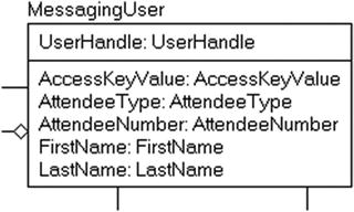
Figure 6-5. MessagingUser table before changing model to use surrogate key
This value is the most logical, but this name, based on the requirements (current and future), can change. Changing this to a surrogate value will make it easier to make the name change and not have to worry about existing data in this table and related tables. Making this change to the model results in the change shown in Figure 6-6, and now, the key is a value that is clearly recognizable as being associated with the MessagingUser, no matter what the uniqueness of the row may be. Note that I made the UserHandle an alternate key as I switched it from primary key.

Figure 6-6. MessagingUser table after changing model to use surrogate key
Next up, we will take a look at the Message table shown in Figure 6-7. Note that the two columns that were named UserHandle and SentToUserHandle have had their role names changed to indicate the change in names from when the key of MessagingUser was UserHandle.

Figure 6-7. Message table before changing model to use surrogate key
We will transform this table to use a surrogate key by moving all three columns to nonkey columns, placing them in a uniqueness constraint, and adding the new MessageId column. Notice, too, in Figure 6-8 that the table is no longer modeled with rounded corners, because the primary key no longer is modeled with any migrated keys in the primary key.

Figure 6-8. Message table before changing model to use surrogate key
Having a common pattern for every table is useful for programming with the tables as well. Because every table has asingle-column key that isn’t updatable and is the same datatype, it’s possible to exploit this in code, making code generation a far more straightforward process. Note once more that nothing should be lost when you use surrogate keys, because a surrogate of this style only stands in for an existing natural key. Many of the object relational mapping (ORM) tools that are popular (if controversial in the database community) require a single-column integer key as their primary implementation pattern. I don’t favor forcing the database to be designed in any manner to suit client tools, but sometimes, what is good for the database is the same as what is good for the tools, making for a relatively happy ending, at least.
By implementing tables using this pattern, I’m covered in two ways: I always have a single primary key value, but I always have a key that cannot be modified, which eases the difficulty for loading a secondary copy like a data warehouse. No matter the choice of human-accessible key, surrogate keys are the style of key that I use for nearly all tables in databases I create (and always for tables with user-modifiable data, which I will touch on when we discuss “domain” tables later in this chapter). In Figure 6-9, I have completed the transformation to using surrogate keys.

Figure 6-9. Messaging Database Model progression after surrogate key choices
Keep in mind that I haven’t specified any sort of implementation details for the surrogate key at this point, and clearly, in a real system, I would already have done this during the transformation. For this chapter example, I am using a deliberately detailed process to separate each individual step, so I will put off that discussion until the DDL section of this book, where I will present code to deal with this need along with creating the objects.
Alternate Keys
In the model so far, we have already identified alternate keys as part of the model creation (MessagingUser.AttendeeNumber was our only initial alternate key), but I wanted to just take a quick stop on the model and make it clear in case you have missed it. Every table should have a minimum of one natural key; that is, a key that is tied to the meaning of what the table is modeling. This step in the modeling process is exceedingly important if you have chosen to do your logical model with surrogates, and if you chose to implement with single part surrogate keys, you should at least review the keys you specified.
A primary key that’s manufactured or even meaningless in the logical model shouldn’t be your only defined key. One of the ultimate mistakes made by people using such keys is to ignore the fact that two rows whose only difference is a system-generated value are not different. With only an artificially generated value as your key, it becomes more or less impossible to tell one row from another.
For example, take Table 6-1, a snippet of a Part table, where PartID is an IDENTITY column and is the primary key for the table.
Table 6-1. Sample Data to Demonstrate How Surrogate Keys Don’t Make Good Logical Keys
|
PartID |
PartNumber |
Description |
|---|---|---|
|
1 |
XXXXXXXX |
The X part |
|
2 |
XXXXXXXX |
The X part |
|
3 |
YYYYYYYY |
The Y part |
How many individual items are represented by the rows in this table? Well, there seem to be three, but are rows with PartIDs 1 and 2 actually the same row, duplicated? Or are they two different rows that should be unique but were keyed in incorrectly? You need to consider at every step along the way whether a human being could not pick a desired row from a table without knowledge of the surrogate key. This is why there should be a key of some sort on the table to guarantee uniqueness, in this case likely on PartNumber.
![]() Caution As a rule, each of your tables should have a natural key that means something to the user and that can uniquely identify each row in your table. In the very rare event that you cannot find a natural key (perhaps, for example, in a table that provides a log of events that could occur in the same .000001 of a second), then it is acceptable to make up some artificial key, but usually, it is part of a larger key that helps you tell two rows apart.
Caution As a rule, each of your tables should have a natural key that means something to the user and that can uniquely identify each row in your table. In the very rare event that you cannot find a natural key (perhaps, for example, in a table that provides a log of events that could occur in the same .000001 of a second), then it is acceptable to make up some artificial key, but usually, it is part of a larger key that helps you tell two rows apart.
In a well-designed logical model, you should not have anything to do at this point with keys that protect the uniqueness of the data from a requirements standpoint. The architect (probably yourself) has already determined some manner of uniqueness that can be implemented. For example, in Figure 6-10, a MessagingUser row can be identified by either the UserHandle or the AttendeeNumber.
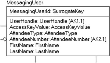
Figure 6-10. MessagingUser table for review
A bit more interesting is the Message table, shown in Figure 6-11. The key is the RoundedMessageTime, which is the time, rounded to the hour, the text of the message, and the UserId.

Figure 6-11. Message table for review
In the business rules, it was declared that the user could not post the same message more than once an hour. Constraints such as this are not terribly easy to implement in a simple manner, but breaking it down to the data you need to implement the constraint can make it easier. In our case, by putting a key on the message, user, and the time rounded to the hour (which we will find some way to implement later in the process), configuring the structures is quite easy.
Of course, by putting this key on the table, if the UI sends the same data twice, an error will be raised when a duplicate message is sent. This error will need to be dealt with at the client side, typically by translating the error message to something nicer.
The last table I will cover here is the MessageTopic table, shown in Figure 6-12.

Figure 6-12. MessageTopic table for review
What is interesting about this table is the optional UserDefinedTopicName value. Later, when we are creating this table, we will load some seed data that indicates that the TopicId is ‘UserDefined’, which means that the UserDefinedTopicName column can be used. Along with this seed data, on this table will be a check constraint that indicates whether the TopicId value represents the user-defined topic. I will use a 0 surrogate key value. In the check constraint later, we will create a check constraint to make sure that all data fits the required criteria.
At this point, to review, we have the model at the point in Figure 6-13.
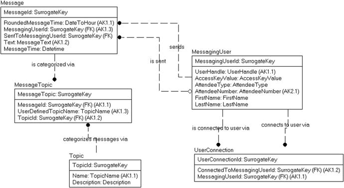
Figure 6-13. Messaging model for review
Determining Domain Implementation
In logical modeling, the concept of domains is used to specify a template for datatypes and column properties that are used over and over again. In physical modeling, domains are used to choose the datatype to use and give us a guide as to the validations we will need to implement.
For example, in the logical modeling phase, domains are defined for such columns as name and description, which occur regularly across a database/enterprise. The reason for defining domains might not have been completely obvious at the time of logical design (it can seem like work to be a pompous data architect, rather than a programmer), but it becomes clear during physical modeling if it has been done well up front. During implementation domains serve several purposes:
- Consistency: We have used TopicName twice as a domain. This reminds us to define every column of type TopicName in precisely the same manner; there will never be any question about how to treat the column.
- Ease of implementation: If the tool you use to model and implement databases supports the creation of domain and template columns, you can simply use the template to build similar columns with the same pattern, and you won’t have to set the values over and over, which leads to mistakes! If you have tool support for property inheritance on domains, when you change a property in the definition, the values change everywhere. So if all descriptive-type columns are nullable, and all code columns are not, you can set this in one place.
- Documentation: Even if every column used a different domain and there was no reuse, the column/domain documentation would be very useful for programmers to be able to see what datatype to use for a given column. In the final section of this chapter, I will include the domain as part of the metadata I will add to the extended properties of the implemented columns.
Domains aren’t a requirement of logical or physical database design, nor does SQL Server actually make it easy for you to use them, but even if you just use them in a spreadsheet or design tool, they can enable easy and consistent design and are a great idea. Of course, consistent modeling is always a good idea regardless of whether you use a tool to do the work for you. I personally have seen a particular column type implemented in four different ways in five different columns when proper domain definitions were not available. So, tool or not, having a data dictionary that identifies columns that share a common type by definition is extremely useful.
For example, for the TopicName domain that’s used often in the Topic and MessageTopic tables in our ConferenceMessage model, the domain may have been specified by the contents of Table 6-2.
Table 6-2. Sample Domain: TopicName
|
Property |
Setting |
|---|---|
|
Name |
TopicName |
|
Optional |
No |
|
Datatype |
Unicode text, 30 characters |
|
Value Limitations |
Must not be empty string or only space characters |
|
Default Value |
n/a |
I’ll defer the CHECK constraint and DEFAULT bits until later in this chapter, where I discuss implementation in more depth. Several tables will have a TopicName column, and you’ll use this template to build every one of them, which will ensure that every time you build one of these columns it will have a type of nvarchar(30). Note that we will discuss data types and their usages later in this chapter.
A second domain that is used very often in our model is SurrogateKey, shown in Table 6-3.
Table 6-3. Sample Domain: SurrogateKey
|
Property |
Setting |
|---|---|
|
Name |
SurrogateKey |
|
Optional |
When used for primary key, not optional, typically auto-generated. When used as a nonkey, foreign key reference, optionality determined by utilization in the relationship. |
|
Datatype |
int |
|
Value Limitations |
N/A |
|
Default Value |
N/A |
This domain is a bit different, in that it will be implemented exactly as specified for a primary key attribute, but when it is migrated for use as a foreign key, some of the properties will be changed. First, if using identity columns for the surrogate, it won’t have the IDENTITY property set. Second, for an optional relationship, an optional relationship will allow nulls in the migrated key, but when used as the primary key, it will not allow them. Finally, let’s set up one more domain definition to our sample, the UserHandle domain, shown in Table 6-4.
Table 6-4. Sample Domain: UserHandle
|
Property |
Setting |
|---|---|
|
Name |
UserHandle |
|
Optional |
no |
|
Datatype |
Basic character set, 20 characters maximum |
|
Value Limitations |
Must be 5–20 simple alphanumeric characters and must start with a letter |
|
Default Value |
n/a |
In the next four subsections, I’ll discuss several topics concerning the implementation of domains:
- Implementing as a column or table: You need to decide whether a value should simply be entered into a column or whether to implement a new table to manage the values.
- Choosing the datatype: SQL Server gives you a wide range of datatypes to work with, and I’ll discuss some of the issues concerning making the right choice.
- Choosing nullability: In this section, I will demonstrate how to implement the datatype choices in the example model.
- Choosing the collation: The collation determines how data is sorted and compared, based on character set and language used.
Getting the domain of a column implemented correctly is an important step in getting the implementation correct. Too many databases end up with all columns with the same datatype and size, allowing nulls (except for primary keys, if they have them), and lose the integrity of having properly sized and constrained constraints.
Enforce Domain in the Column, or With a Table?
Although many domains have only minimal limitations on values, often a domain will specify a fixed set of named values that a column might have that is less than can be fit into one of the base datatypes. For example, in the demonstration table MessagingUser shown in Figure 6-14, a column AttendeeType has a domain of AttendeeType.

Figure 6-14. MessageUser table for reference
This domain might be specified as in Table 6-5.
Table 6-5. Genre Domain
|
Property |
Setting |
|---|---|
|
Name |
AttendeeType |
|
Optional |
No |
|
Datatype |
Basic character set, maximum 20 characters |
|
Value Limitations |
Regular, Volunteer, Speaker, Administrator |
|
Default Value |
Regular |
The value limitation limits the values to a fixed list of values. We could choose to implement the column using a declarative control (a CHECK constraint, which we will cover in more detail later in the chapter) with a predicate of AttendeeType IN (’Regular’, ’Volunteer’, ’Speaker’, ’Administrator’) and a literal default value of ’Regular’. There are a couple of minor annoyances with this form:
- There is no place for table consumers to know the domain: Unless you have a row with one of each of the values and you do a DISTINCT query over the column (something that is generally poorly performing), it isn’t easy to know what the possible values are without either having foreknowledge of the system or looking in the metadata. If you’re doing Conference Messaging system utilization reports by AttendeeType, it won’t be easy to find out what attendee types had no activity for a time period, certainly not using a simple, straightforward SQL query that has no hard-coded values.
- Often, a value such as this could easily have additional information associated with it: For example, this domain might have information about actions that a given type of user could do. For example, if a Volunteer attendee is limited to using certain topics, you would have to manage the types in a different table. Ideally, if you define the domain value in a table, any other uses of the domain are easier to maintain.
I nearly always include tables for all domains that are essentially “lists” of items, as it is just far easier to manage, even if it requires more tables. The choice of key for a domain table can be a bit different than for most tables. Sometimes, I use a surrogate key for the actual primary key, and other times, I use a natural key. The general difference is whether or not the values are user manageable, and if the programming tools require the integer/GUID approach (for example, if the front-end code uses an enumeration that is being reflected in the table values). In the model, I have two examples of such types of domain implementations. In Figure 6-15, I have added a table to implement the domain for attendee types, and for this table, I will use the natural key.

Figure 6-15. AttendeeType domain implemented as a table
This lets an application treat the value as if it is a simple value just like if this was implemented without the domain table. So if the application wants to manage the value as a simple string value, I don’t have to know about it from the database standpoint. I still get the value and validation that the table implementation affords me, plus the ability to have a Description column describing what each of the values actually means (which really comes in handy at 12:10 AM on December the 25th when the system is crashing and needs to be fixed, all while you are really thinking about the bicycle you haven’t finished putting together).
In the original model, we had the Topic table, shown in Figure 6-16, which is a domain similar to the AttendeeType but is designed to allow a user to make changes to the topic list.
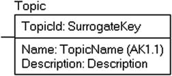
Figure 6-16. Topic table for reference
The Topic entity has the special case that it can be added to by the application managers, so it will be implemented as a numeric surrogate value. We will initialize the table with a row that represents the user-defined topic that allows the user to enter their own topic in the MessageTopic table.
Choosing the Datatype
Choosing proper datatypes to match the domain chosen during logical modeling is an important task. One datatype might be more efficient than another of a similar type. For example, you can store integer data in an integer datatype, a numeric datatype, a floating-point datatype, or even a varchar(10) type, but these datatypes are certainly not alike in implementation or performance.
![]() Note I have broken up the discussion of datatypes into two parts. First, there is this and other sections in this chapter in which I provide some basic guidance on the types of datatypes that exist for SQL Server and some light discussion on what to use. Appendix A at the end of this book is an expanded look at all of the datatypes and is dedicated to giving examples and example code snippets with all the types.
Note I have broken up the discussion of datatypes into two parts. First, there is this and other sections in this chapter in which I provide some basic guidance on the types of datatypes that exist for SQL Server and some light discussion on what to use. Appendix A at the end of this book is an expanded look at all of the datatypes and is dedicated to giving examples and example code snippets with all the types.
It’s important to choose the best possible datatype when building the column. The following list contains the intrinsic datatypes (built-in types that are installed when you install SQL Server) and a brief explanation of each of them. As you are translating domains to implementation, step 1 will be to see which of these types matches to need best first, then we will look to constrain the data even further with additional techniques.
- Precise numeric data: Stores numeric data with no possible loss of precision.
- bit: Stores either 1, 0, or NULL; frequently used for Boolean-like columns (1 = True, 0 = False, NULL = Unknown). Up to 8-bit columns can fit in 1 byte. Some typical integer operations, like basic math, cannot be performed.
- tinyint: Non-negative values between 0 and 255 (0 to 2^8 - 1) (1 byte).
- smallint: Integers between –32,768 and 32,767 (-2^15 to 2^15 – 1) (2 bytes).
- int: Integers between -2,147,483,648 and 2,147,483,647 (–2^31 to 2^31 – 1) (4 bytes).
- bigint: Integers between 9,223,372,036,854,775,808 and 9,223,372,036,854,775,807 (-2^63 to 2^63 – 1) (8 bytes).
- decimal (or numeric, which is functionally the same in SQL Server, but decimal is generally preferred for portability): All numbers between –10^38 – 1 and 10^38 – 1 (between 5 and 17 bytes, depending on precision). Allows for fractional numbers, unlike integer-suffixed types.
- Approximate numeric data: Stores approximations of numbers, typically for scientific usage. Gives a large range of values with a high amount of precision but might lose precision of very large or very small numbers.
- float(N): Values in the range from –1.79E + 308 through 1.79E + 308 (storage varies from 4 bytes for N between 1 and 24, and 8 bytes for N between 25 and 53).
- real: Values in the range from –3.40E + 38 through 3.40E + 38. real is an ISO synonym for a float(24) datatype, and hence equivalent (4 bytes).
- Date and time: Stores values that deal with temporal data.
- date: Date-only values from January 1, 0001, to December 31, 9999 (3 bytes).
- time: Time-of-day-only values to 100 nanoseconds (3 to 5 bytes).
- datetime2(N): Despite the hideous name, this type will store a point in time from January 1, 0001, to December 31, 9999, with accuracy ranging from 1 second (0) to 100 nanoseconds (7) (6 to 8 bytes).
- datetimeoffset: Same as datetime2, but includes an offset for time zone (8 to 10 bytes).
- smalldatetime: A point in time from January 1, 1900, through June 6, 2079, with accuracy to 1 minute (4 bytes). (Note: It is suggested to phase out usage of this type and use the more standards-oriented datetime2, though smalldatetime is not technically deprecated.)
- datetime: Points in time from January 1, 1753, to December 31, 9999, with accuracy to 3.33 milliseconds (8 bytes). (Note: It is suggested to phase out usage of this type and use the more standards-oriented datetime2, though datetime is not technically deprecated.)
- Binary data: Strings of bits, for example, files or images. Storage for these datatypes is based on the size of the data stored.
- binary(N): Fixed-length binary data up to 8,000 bytes long.
- varbinary(N): Variable-length binary data up to 8,000 bytes long.
- varbinary(max): Variable-length binary data up to (2^31) – 1 bytes (2GB) long.
- Character (or string) data:
- char(N): Fixed-length character data up to 8,000 characters long.
- varchar(N): Variable-length character data up to 8,000 characters long.
- varchar(max): Variable-length character data up to (2^31) – 1 bytes (2GB) long.
- nchar, nvarchar, nvarchar(max): Unicode equivalents of char, varchar, and varchar(max).
- Other datatypes:
- sql_variant: Stores (pretty much) any datatype, other than CLR-based datatypes (hierarchyId, spatial types) and any types with a max length of over 8,016 bytes. (CLR is a topic I won’t hit on too much, but it allows Microsoft and you to program SQL Server objects in a .NET language. For more information, check https://msdn.microsoft.com/en-us/library/ms131089.aspx). It’s generally a bad idea to use sql_variant for all but a few fringe uses. It is usable in cases where you don’t know the datatype of a value before storing. The only use of this type in the book will be in Chapter 8 when we create user-extensible schemas (which is itself a fringe pattern.)
- rowversion (timestamp is a synonym): Used for optimistic locking to version-stamp a row. It changes on every modification. The name of this type was timestamp in all SQL Server versions before 2000, but in the ANSI SQL standards, the timestamp type is equivalent to the datetime datatype. I’ll make further use of the rowversion datatype in more detail in Chapter 11, which is about concurrency. (16 years later, and it is still referred to as timestamp very often, so this may never actually go away completely.)
- uniqueidentifier: Stores a GUID value.
- XML: Allows you to store an XML document in a column. The XML type gives you a rich set of functionality when dealing with structured data that cannot be easily managed using typical relational tables. You shouldn’t use the XML type as a crutch to violate First Normal Form by storing multiple values in a single column. I will not use XML in any of the designs in this book.
- Spatial types (geometry, geography, circularString, compoundCurve, and curvePolygon): Used for storing spatial data, like for maps. I will not be using these types in this book.
- hierarchyId: Used to store data about a hierarchy, along with providing methods for manipulating the hierarchy. We will cover more about manipulating hierarchies in Chapter 8.
Choice of datatype is a tremendously important part of the process, but if you have defined the domain well, it is not that difficult of a task. In the following sections, we will look at a few of the more important parts of the choice. A few of the considerations we will include are
- Deprecated or bad choice types
- Common datatype configurations
- Large-value datatype columns
- Complex datatypes
I didn’t use too many of the different datatypes in the sample model, because my goal was to keep the model very simple and not try to be an AdventureWorks-esque model that tries to show every possible type of SQL Server in one model (or even the newer WideWorldImporters database, which is less unrealistically complex than AdventureWorks and will be used in several chapters later in the book).
Deprecated or Bad Choice Types
I didn’t include several datatypes in the previous list because they have been deprecated for quite some time, and it wouldn’t be surprising if they are completely removed from the version of SQL Server after 2016 (even though I said the same thing in the previous few versions of the book, so be sure to stop using them as soon as possible). Their use was common in versions of SQL Server before 2005, but they’ve been replaced by types that are far easier to use:
- image: Replace with varbinary(max)
- text or ntext: Replace with varchar(max) and nvarchar(max)
If you have ever tried to use the text datatype in SQL code, you know it is not a pleasant thing. Few of the common text operators were implemented to work with it, and in general, it just doesn’t work like the other native types for storing string data. The same can be said with image and other binary types. Changing from text to varchar(max), and so on, is definitely a no-brainer choice.
The second types that are generally advised against being used are the two money types:
- money: –922,337,203,685,477.5808 through 922,337,203,685,477.5807 (8 bytes)
- smallmoney: Money values from –214,748.3648 through 214,748.3647 (4 bytes)
In general, the money datatype sounds like a good idea, but using it has some confusing consequences. In Appendix A, I spend a bit more time covering these consequences, but here are two problems:
- There are definite issues with rounding off, because intermediate results for calculations are calculated using only four decimal places.
- Money data input allows for including a monetary sign (such as $ or £), but inserting $100 and £100 results in the same value being represented in the variable or column.
Hence, it’s generally accepted that it’s best to store monetary data in decimal datatypes. This also gives you the ability to assign the numeric types to sizes that are reasonable for the situation. For example, in a grocery store, having the maximum monetary value of a grocery item over 200,000 dollars is probably unnecessary, even figuring for a heck of a lot of inflation. Note that in the appendix I will include a more thorough example of the types of issues you could see.
Common Datatype Configurations
In this section, I will briefly cover concerns and issues relating to Boolean/logical values, large datatypes, and complex types and then summarize datatype concerns in order to discuss the most important thing you need to know about choosing a datatype.
Boolean values (TRUE or FALSE) are another of the hotly debated choices that are made for SQL Server data. There’s no Boolean type in standard SQL, since every type must support NULL, and a NULL Boolean makes life far more difficult for the people who implement SQL, so a suitable datatype needs to be chosen through which to represent Boolean values. Truthfully, though, what we really want from a Boolean is the ability to say that the property of the modeled entity “is” or “is not” for some basic setting.
There are three common choices to implement a value of this sort:
- Using a bit datatype where a value of 1:True and 0:False: This is, by far, the most common datatype because it works directly with programming languages such as the .NET languages with no translation. The check box and option controls can directly connect to these values, even though a language like VB used -1 to indicate True. It does, however, draw the ire of purists, because it is too much like a Boolean. Commonly named “flag” as a classword, like for a special sale indicator: SpecialSaleFlag. Some people who don’t do the suffix thing as a rule often start the name off with Is, like IsSpecialSale. Microsoft uses the prefix in the catalog views quite often, like in sys.databases: is_ansi_nulls_on, is_read_only, and so on.
- A char(1) value with a domain of ’Y’, ’N’; ’T’, ’F’, or other values: This is the easiest for ad hoc users who don’t want to think about what 0 or 1 means, but it’s generally the most difficult from a programming standpoint. Sometimes, a char(3) is even better to go with ’yes’ and ’no’. Usually named the same as the bit type, but just having a slightly more attractive looking output.
- A full, textual value that describes the need: For example, a preferred customer indicator, instead of PreferredCustomerFlag, PreferredCustomerIndicator, with values ’Preferred Customer’ and ’Not Preferred Customer’. Popular for reporting types of databases, for sure, it is also more flexible for when there becomes more than two values, since the database structure needn’t change if you need to add ’Sorta Preferred Customer’ to the domain of PreferredCustomerIndicator.
As an example of a Boolean column in our messaging database, I’ll add a simple flag to the MessagingUser table that tells whether the account has been disabled, as shown in Figure 6-17. As before, we are keeping things simple, and in simple cases, a simple flag might do it. But of course, in a sophisticated system, you would probably want to have more information, like who did the disabling, why they did it, when it took place, and perhaps even when it takes effect (these are all questions for design time, but it doesn’t hurt to be thorough).

Figure 6-17. MessagingUser table with DisabledFlag bit column
In SQL Server 2005, dealing with large datatypes changed quite a bit (and hopefully someday Microsoft will kill the text and image types for good). By using the max specifier on varchar, nvarchar, and varbinary types, you can store far more data than was possible in previous versions using a “normal” type, while still being able to deal with the data using the same functions and techniques you can on a simple varchar(10) column, though performance will differ slightly.
As with all datatype questions, use the varchar(max) types only when they’re required, always use the smallest types possible. The larger the datatype, the more data possible, and the more trouble the row size can be to get optimal storage retrieval times. In cases where you know you need large amounts of data or in the case where you sometimes need greater than 8,000 bytes in a column, the max specifier is a fantastic thing.
![]() Note Keep on the lookout for uses that don’t meet the normalization needs, as you start to implement. Most databases have a “comments” column somewhere that morphed from comments to a semistructured mess that your DBA staff then needs to dissect using SUBSTRING and CHARINDEX functions.
Note Keep on the lookout for uses that don’t meet the normalization needs, as you start to implement. Most databases have a “comments” column somewhere that morphed from comments to a semistructured mess that your DBA staff then needs to dissect using SUBSTRING and CHARINDEX functions.
There are two special concerns when using these types:
- There’s no automatic datatype conversion from the normal character types to the large-value types.
- Because of the possible large sizes of data, a special clause is added to the UPDATE statement to allow partial column modifications.
The first issue is pretty simple, but it can be a bit confusing at times. For example, concatenate ’12345’ + ’67890’. You’ve taken two char(5) values, and the result will be contained in a value that is automatically recast as a char(10). But if you concatenate two varchar(8000) values, you don’t get a varchar(16000) value, and you don’t get a varchar(max) value. The values get truncated to a varchar(8000) value. This isn’t always intuitively obvious. For example, consider the following code:
SELECT   LEN( CAST(REPLICATE (’a’,8000) AS varchar(8000))
            + CAST(REPLICATE(’a’,8000) AS varchar(8000))
          )
It returns a value 8000, as the two columns concatenate to a type of varchar(8000). If you cast one of the varchar(8000) values to varchar(max), then the result will be 16,000:
SELECT    LEN(CAST(REPLICATE(’a’,8000) AS varchar(max))
            + CAST(REPLICATE(’a’,8000) AS varchar(8000))
          )
Second, because the size of columns stored using the varchar(max) datatype can be so huge, it wouldn’t be favorable to always pass around these values just like you do with smaller values. Because the maximum size of a varchar(max) value is 2GB, imagine having to update a value of this size in its entirety. Such an update would be pretty nasty, because the client would need to get the whole value, make its changes, and then send the value back to the server. Most client machines may only have 2GB of physical RAM, so paging would likely occur on the client machine, and the whole process would crawl and more than likely crash occasionally. So, you can do what are referred to as chunked updates. These are done using the .WRITE clause in the UPDATE statement. For example:
UPDATE TableName
SET    VarcharMaxCol.WRITE(’the value’, <offset>, <expression>)
WHERE  . . .
One important thing to note is that varchar(max) values will easily cause the size of rows to be quite large. In brief, a row that fits into 8,060 bytes can be stored in one physical unit. If the row is larger than 8,060 bytes, string data can be placed on what are called overflow pages. Overflow pages are not terribly efficient because SQL Server has to go fetch extra pages that will not be in line with other data pages. (Physical structures, including overflow pages, are covered more in Chapter 10 when the physical structures are covered.)
I won’t go over large types in any more detail at this point. Just understand that you might have to treat the data in the (max) columns differently if you’re going to allow huge quantities of data to be stored. In our model, we’ve used a varbinary(max) column in the Customer table to store the image of the customer.
The main point to understand here is that having a datatype with virtually unlimited storage comes at a price. Versions of SQL Server starting in 2008 allow you some additional freedom when dealing with varbinary(max) data by placing it in the file system using what is called filestream storage. I will discuss large object storage in Chapter 8 in more detail, including file tables.
One really excellent sounding feature that you can use to help make your code cleaner is a user-defined type (UDT), which is really an alias to a type. You can use a datatype alias to specify a commonly used datatype configuration that’s used in multiple places using the following syntax:
CREATE TYPE <typeName>
        FROM <intrinsic type> --any type that can be used as a column of a
                              --table, with precision and scale or length,
                              --as required by the intrinsic type
        [NULL | NOT NULL];
When declaring a table, if nullability isn’t specified, then NULL or NOT NULL is based on the setting of ANSI_NULL_DFLT_ON, except when using an alias type (variables will always be nullable). In general, it is best to always specify the nullability in the table declaration, and something I will do always in the book, though I do sometimes forget in real life.
For example, consider the UserHandle column. Earlier, we defined its domain as being varchar(20), not optional, alphanumeric, with the data required to be between 5 and 20 characters. The datatype alias would allow us to specify
CREATE TYPE UserHandle FROM varchar(20) NOT NULL;
Then, in the CREATE TABLE statement, we could specify
CREATE TABLE MessagingUser
...
UserHandle UserHandle,
By declaring that the UserHandle type will be varchar(20), you can ensure that every time the type of UserHandle is used, in table declarations, and variable declarations will be varchar(20) and as long as you don’t specify NULL or NOT NULL. It is not possible to implement the requirement that data be between 5 and 20 characters on any other constraints on the type, including the NULL specification.
For another example, consider an SSN type. It’s char(11), so you cannot put a 12-character value in, sure. But what if the user had entered 234433432 instead of including the dashes? The datatype would have allowed it, but it isn’t what’s desired. The data will still have to be checked in other methods such as CHECK constraints.
I am personally not a user of these types. I have never really used these kinds of types because of the fact that you cannot do anything with these other than simply alias a type. Any changes to the type also require removal of all references to the type making a change to the type a two step process.
I will note, however, that I have a few architect friends who make extensive use of them to help keep data storage consistent. I have found that using domains and a data modeling tool serves me better, but I do want to make sure that you have at least heard of them and know the pros and cons.
In SQL Server 2005 and later, we can build our own datatypes using the SQL CLR (Common Language Runtime). Unfortunately, they are quite cumbersome, and the implementation of these types does not lend itself to the types behaving like the intrinsic types. Utilizing CLR types will require you to install the type on the client for them to get the benefit of the type being used.
For the most part you should use CLR types only in the cases where it makes a very compelling reason to do so. There are a few different possible scenarios where you could reasonably use user-defined types to extend the SQL Server type system with additional scalar types or different ranges of data of existing datatypes. Some potential uses of UDTs might be
- Complex types that are provided by an owner of a particular format, such as a media format that could be used to interpret a varbinary(max) value as a movie or an audio clip. This type would have to be loaded on the client to get any value from the datatype.
- Complex types for a specialized application that has complex needs, when you’re sure your application will be the only user.
Although the possibilities are virtually unlimited, I suggest that CLR UDTs be considered only for specialized circumstances that make the database design extremely more robust and easy to work with. CLR UDTs are a nice addition to the DBA’s and developer’s toolkit, but they should be reserved for those times when adding a new scalar datatype solves a complex business problem.
Microsoft has provided several intrinsic types based on the CLR to implement hierarchies and spatial datatypes. I point this out here to note that if Microsoft is using the CLR to implement complex types (and the spatial types at the very least are pretty darn complex), the sky is the limit. I should note that the spatial and hierarchyId types push the limits of what should be in a type, and some of the data stored (like a polygon) is more or less an array of connected points.
Choosing the Right Datatype
SQL Server gives you a wide range of datatypes, and many of them can be declared in a wide variety of sizes. I never cease to be amazed by the number of databases around in which every single column is either an integer or a varchar(N) (where N is the same for every single string column, sometimes in the 8000 range) and varchar(max). One particular example I’ve worked with had everything, including GUID-based primary keys, all stored in NVARCHAR(200) columns! It is bad enough to store your GUIDs in a varchar column at all, since it can be stored as a 16-byte binary value, whereas if you use a varchar column, it will take 36 bytes; however, store it in an nvarchar (Unicode) column, and now it takes 72 bytes! What a terrible waste of space. Even worse, someone could put in a non-GUID value up to 200 characters wide. Now, people using the data will feel like they need to allow for 200 characters on reports and such for the data. Time wasted, space wasted, money wasted.
As another example, say you want to store a person’s name and date of birth. You could choose to store the name in a varchar(max) column and the date of birth in a varchar(max) column. In all cases, these choices would certainly store the data that the user wanted, but they wouldn’t be good choices at all. The name should be in something such as a nvarchar(50) column and the date of birth in a date column. Notice that I used a variable-sized type for the name. This is because you don’t know the length, and not all names are the same size. Because most names aren’t nearly 50 bytes, using a variable-sized type will save space in your database. I used a Unicode type because person’s names do actually fit the need of allowing nontypical Latin characters.
Of course, in reality, seldom would anyone make such poor choices of a datatype as putting a date value in a varchar(max) column. Most choices are reasonably easy. However, it’s important to keep in mind that the datatype is the first level of domain enforcement. Thinking back to our domain for UserHandle, we had the datatype definition and value limitations specified in Table 6-6.
Table 6-6. Sample Domain:UserHandle
|
Property |
Setting |
|---|---|
|
Name |
UserHandle |
|
Optional |
no |
|
Datatype |
Basic character set, maximum 20 characters |
|
Value Limitations |
Must be 5-20 simple alphanumeric characters and start with a letter |
|
Default Value |
n/a |
You can enforce the first part of this at the database level by declaring the column as a varchar(20). A column of type varchar(20) won’t even allow a 21-character or longer value to be entered. It isn’t possible to enforce the rule of greater than or equal to five characters using only a datatype. I’ll discuss more about how to enforce simple domain requirements later in this chapter, and in Chapter 7 I’ll discuss patterns of integrity enforcement that are more complex. In this case, I do use a simple ASCII character set because the requirements called for simple alphanumeric data.
Initially, we had the model in Figure 6-18 for the MessagingUser table.

Figure 6-18. MessagingUser table before choosing exact datatypes
Choosing types, we will use an int for the surrogate key (and in the DDL section, we will set the implementation of the rest of the optionality rule set in the domain: “Not optional auto-generated for keys, optionality determined by utilization for nonkey”, but will replace items of SurrogateKey domain with int types. User handle was discussed earlier in this section. In Figure 6-19, I chose some other basic types for Name. AccessKeyValue, and the AttendeeType columns.

Figure 6-19. MessagingUser after datatype choice
Sometimes, you won’t have any real domain definition, and you will use common sizes. For these, I suggest using either a standard type (if you can find them, like on the Internet) or look through data you have in your system. Until the system gets into production, changing types is fairly easy from a database standpoint, but the more code that accesses the structures the more difficult it gets to make changes.
For the Message table in Figure 6-20, we will choose types.

Figure 6-20. Message table before datatype choice
The text column isn’t datatype text but is the text of the message, limited to 200 characters. For the time columns, in Figure 6-21, I choose datetime2(0) for the MessageTime, since the requirements specified time down to the second. For RoundedMessageTime, we will be rounding to the hour, and so I chose also will expect it to be datetime2(0), though it will be a calculated column based on the MessageTime value. Hence, MessageTime and RoundedMessageTime are two views of the same data value.

Figure 6-21. Message table after datatype choice, with calculated column denoted
So, I am going to use a calculated column as shown in Figure 6-21. I will specify the type of RoundedMessageTime as a nonexistent datatype (so if I try to create the table, it will fail). A calculated column is a special type of column that isn’t directly modifiable, as it is based on the result of an expression.
Later in this chapter, we will specify the actual implementation, but for now, we basically just set a placeholder. Of course, in reality, I would specify the implementation immediately, but again, for this first learning process, I am doing things in this deliberate manner to keep things orderly. So, in Figure 6-22, I have the model with all of the datatypes set.
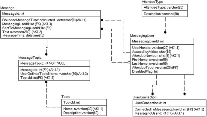
Figure 6-22. Messaging system model after datatype choices
The next step in the process is to set nullability of columns. In our domains, we specified if the columns were optional, so this will generally be a simple task. For the Message table in Figure 6-23, I have chosen the following nullability settings for the columns.

Figure 6-23. Message table for review
The interesting choice was for the two MessagingUserId columns. In Figure 6-24, you can see the full model, but note the relationships from MessagingUser to Message. The relationship for the user that sent the message (MessagingUserId) is NOT NULL, because every message is sent by a user. However, the relationship representing the user the message was sent to is nullable, since not every message needs to be sent to a user.

Figure 6-24. Messaging system model, with NULLs chosen
At this point, our model is very nearly done and very much resembles a database that could be built and employed in an application. Just a bit more information is needed to finish out the model.
The collation of a string value sets up the way a string is compared with another string, as well as how they are sorted. Many character sets are used by the many different cultures around the world. While you can choose a Unicode datatype if you need to store the characters for almost any character set, there still is the question of how data is sorted (case sensitive or not) and compared (accent sensitive or not). SQL Server and Windows provide a tremendous number of collation types to choose from. The collation is specified at many levels, starting with the server. The server collation determines how much of the system metadata is stored. Then the database has a collation, and finally, each column may have a different collation.
It’s a somewhat uncommon need for the average database to change the collation from the default, which is usually chosen to be the most typical for all users of a system. This is usually a case-insensitive collation, which allows that when doing comparisons and sorts, ’A’ = ’a’. I’ve only used an alternative collation a few times for columns where case sensitivity was desired (one time was so that a client could force more four-character codes than a case-insensitive collation would allow!).
To see the current collation type for the server and database, you can execute the following commands:
SELECT SERVERPROPERTY(’collation’);
SELECT DATABASEPROPERTYEX(’DatabaseName’,’collation’);
On most systems installed in English-speaking countries, the default collation type is SQL_Latin1_General_CP1_CI_AS, where Latin1_General represents the normal Latin alphabet, CP1 refers to code page 1252 (the SQL Server default Latin 1 ANSI character set), and the last parts represent case insensitive and accent sensitive, respectively. You can find full coverage of all collation types in the SQL Server documentation. However, the default is rarely the desired collation to use, and is set to that older collation for backward compatibility. Ideally, you will use a Windows collation, and I will use Latin1_General_100_CI_AS for my example code, which will be what I have installed my server as. The 100 indicates this is a newer collation that supports later Unicode characters.
In addition to the normal collations, there are also binary collations that you can use to sort and compare data based on in its raw format. There are two types of binary collations: the older ones are suffixed _bin, and newer ones _bin2. Bin2 collations do what is referred to as pure code-point collations, meaning they compare data only on the binary value (the bin collation compared the first byte as a WCHAR, which is an OLEDB datatype). Note that there will be a difference between binary sort order and case sensitive, so it will behoove you to take some time to understand the collation that you end up using.
To list all the sort orders installed in a given SQL Server instance, you can execute the following statement:
SELECT *
FROM ::fn_helpcollations();
On the computer on which I do testing, this query returned more than 3,800 rows, but usually, you don’t need to change from the default that the database administrator initially chooses. To set the collation sequence for a char, varchar, text, nchar, nvarchar, or ntext column when creating a column, you specify it using the COLLATE clause of the column definition, like so:
CREATE SCHEMA alt;
CREATE TABLE alt.OtherCollate
(
   OtherCollateId int IDENTITY
        CONSTRAINT PKAlt_OtherCollate PRIMARY KEY ,
   Name nvarchar(30) NOT NULL,
   FrenchName nvarchar(30) COLLATE French_CI_AS_WS NULL,
   SpanishName nvarchar(30) COLLATE Modern_Spanish_CI_AS_WS NULL
);
Now, when you sort output by FrenchName, it’s case insensitive, but arranges the rows according to the order of the French language. The same applies with Spanish, regarding the SpanishName column. For this chapter we will stick with the default in almost all cases, and I would suggest taking a look at Books Online if you have the need to store data in multiple languages. The only “normal” variation from the default collation of the database is if you need a different case sensitivity for a column, in which case you might use a binary collation, or a case sensitive one.
One quick note, you can specify the collation in a WHERE clause using the COLLATE keyword:
SELECT Name
FROM alt.OtherCollate
WHERE Name COLLATE Latin1_General_CS_AI
           LIKE ’[A-Z]%’ collate Latin1_General_CS_AI;  --case sensitive and
                                                        --accent insensitive
It is important to be careful when choosing a collation that is different from the default, because at the server level it is extremely hard to change, and at the database level it is no picnic. You can change the collation of a column with an ALTER command, but it can’t have constraints or indexes referencing it, and you may need to recompile all of your objects that reference the tables.
If you do find yourself on a server with multiple collations, a handy collation setting to use can be database_default, which uses the default for the context of the database you are executing from.
It is important to choose your collation wisely when setting up a server, database, table, etc. Changing the collation of a database can be done using a simple ALTER statement. However, it will not change any objects in the database. You will have to change every column’s collation individually, and while you can use a simple ALTER TABLE…ALTER COLUMN statement to change the collation, you will have to drop all indexes, constraints, and schema-bound objects that reference the column first. It is a pretty painful task.
A schema is a namespace: a container where database objects are contained, all within the confines of a database. We will use schemas to group our tables and eventually views, procedures, functions, etc. into functional groups. Naming schemas is a bit different than naming tables or columns. Schema names should sound right, so sometimes, they make sense to be plural, and other times singular. It depends on how they are being used. I find myself using plural names most of the time because it sounds better, and because sometimes, you will have a table named the same thing as the schema if both were singular.
In our model in Figure 6-25, we will put the tables that are used to represent messages in a Messages schema, and the ones that represent Attendees and their relationships to one another in a schema we will name Attendees.

Figure 6-25. Messages model with schemas assigned
Note, too, that I often will set up schemas late in the process, and it might seem more correct to start there. I find that it is often easier to discover the different areas of the implementation, and that schemas aren’t necessarily easy to start with, but that different areas come and go until I get to the final solution. Sometimes, it is by necessity because you have multiple tables with the same name, though this can be a sign of a bad design. In this manufactured solution, I simply did it last to make the point that it could be last.
What makes schemas so nice is that you can deal with permissions on a schema level, rather than on an object-by-object level. Schemas also give you a logical grouping of objects when you view them within a list, such as in Management Studio.
I’m not going to go any further into the security aspects of using schemas at this point in the book, but understand that schemas are not just for aesthetics. Throughout this book, I’ll always name the schema that a table is in when doing examples. Schemas will be part of any system I design in this book, simply because it’s going to be best practice to do so. On a brief trip back to the land of reality, I said in the previous editions of this book that beginning to use schemas in production systems will be a slow process, and it still can be jarring to some users 11+ years later. Chapter 9 will discuss using schemas for security in more detail.
Finally, I will add one more thing to the database: columns to support the implementation of the code only (and not to support a user requirement directly). A very common use is to have columns that indicate when the row was created, when it was updated, and perhaps by whom. In our model, I will stick to the simple case of the times mentioned and will demonstrate how to implement this in the database. A lot of implementers like to leave these values to the client, but I very much prefer using the database code because then I have one clock managing times, rather than multiples. (I once managed a system that used two clocks to set row times, and occasionally a row was created years after it was last updated!)
So in Figure 6-26, I add two NOT NULL columns to every table for the RowCreateTime and RowLastUpdateTime, except for the AttendeeType table, which we specified to be not user manageable, and so I chose not to include the modified columns for that table. Of course, you might want to do this to let your development team know when the row was first available. I also left off columns to denote who changed the row for simplicity.

Figure 6-26. Message model after adding RowCreateTime and RowLastUpdateTime to tables
As a final note, it is generally best to only use these implementation columns strictly for metadata purposes. For example, consider the Messages.Message table. If you need to know when the message was created, you should use the MessageTime column as that value may represent the time when the user clicked the create button, captured from a different clock source, even if it took five minutes to actually store the data. Plus, if you need to load the data into a new table, the row may have been created in 2016, but the data in 2000, so not using these columns as user data means you can truthfully reflect when the row was created.
That is why I use such clunky names for the implementation column. Many tables will include the creation time, but that data may be modifiable. I don’t want users changing the time when the row was created, so the name notes that the time of creation is strictly for the row, and I don’t allow this column to be modified by anyone.
Sometimes, I will use these columns in concurrency control to denote when a row was changed, but when I have control over the design, I will use a rowversion type if the client can (and will) make use of it. Concurrency control is a very important topic that I will spend a full chapter on in Chapter 11.
Using DDL to Create the Database
So far, we have been molding the model to make it fit our needs to implement. We added columns, added tables, and specified constraints. Now, in this latter half of the chapter, we move toward the mechanical bits of the process, in that all that’s left is to implement the tables we have spent so much time designing. The blueprints have been drawn up, and now, we can finally grab a hammer and start driving nails.
Just like in the rest of this book, I’ll do this work manually using DDL, because it will help you understand what a tool is building for you. It’s also a good exercise for any database architect or DBA to review the SQL Server syntax; I personally wouldn’t suggest building a database with 300 tables without a data modeling tool, but I definitely do know people who do and wouldn’t consider using a tool to create any of their database objects. On the other hand, the same data modeling tools that could be used to do the logical modeling can usually create the tables and often some of the associated code, saving your fingers from added wear and tear, plus giving you more time to help Mario save the princess who always seems to get herself captured. No matter how you do the work, you need to make sure that you end up with scripts of DDL that you or the tool uses to create objects in some manner in the file system, because they’re invaluable tools for the DBA to apply changes to production, test, development, QA, or whatever environments have been set up to allow developers, users, and DBAs to coexist throughout the process.
Make sure that your scripts are in a source control system too, or at the very least backed up. In SQL Server, we have two tools that we can work in, Management Studio and Visual Studio Data Tools. Data Tools is the development-oriented tool that allows a developer to work in a manner kind of like a .Net developer would. Management Studio is more administrative oriented in its toolset, but has tools to view and edit objects directly.
In this book, I am going to stick to the DDL that any of the tools will use to construct objects using an online paradigm where I create a database directly one command at a time. Such scripts can be executed using any SQL Server tool, but I will generally just use a query window in Management Studio, or sometimes the SQLCMD.exe command-line tools when executing multiple scripts. You can download Management Studio or Data Tools from the Microsoft web site for free at msdn.microsoft.com/library/mt238290.aspx or msdn.microsoft.com/en-us/library/mt204009.aspx, respectively, though these locations are certainly apt to change in the years after this book is released.
Before starting to build anything else, you’ll need a database. I’ll create this database using all default values, and my installation is very generic on a Hyper-V VM on my laptop (most any VM technology will do, or you can install on most modern versions of Windows; and as of this writing, a version of SQL Server running on Linux is being previewed, and the crust of the earth has not frozen over). I use the Developer Edition, and I used most of the default settings when installing (other than setting up mixed mode for security to allow for some security testing later, and the collation, which I will set to Latin1_General_100_CI_AS), which will not be optimal when setting up a server for real multiuser use, or if you want to test features like Always On, Replication, etc. All users of a server for the material I am presenting can be managed and created in SQL Server code alone.
If you are using a shared server, such as a corporate development server, you’ll need to do this with an account that has rights to create a database. If you install your server yourself, part of the process will be to set up users so the server will be accessible.
Choosing a database name is in the same level of importance as naming of other objects, and I tend to take the same sort of naming stance. Keep it as simple as possible to differentiate between all other databases, and follow the naming standards in place for your organization. I would try to be careful to try to standardize names across instances of SQL Server to allow moving of databases from server to server. In the code downloads, I will name the database ConferenceMessaging.
The steps I’ll take along the way are as follows:
- Creating the basic table structures: Building the base objects with columns.
- Adding uniqueness constraints: Using primary and unique constraints to enforce uniqueness between rows in the table.
- Building default constraints: Assisting users in choosing proper values when it isn’t obvious.
- Adding relationships: Defining how tables relate to one another (foreign keys).
- Implementing Basic Check Constraints: Some domains need to be implemented a bit more strictly than using a simple datatype.
- Documenting the database: Including documentation directly in the SQL Server objects.
- Validating the dependency information: Using the catalog views and dynamic management views, you can validate that the objects you expect to depend on the existence of one another do, in fact, exist, keeping your database cleaner to manage.
I will use the following statement to create a small database: CREATE DATABASE ConferenceMessaging; You can see where the database files were placed by running the following statement (note that size is presented in 8KB pages—more on the internal structures of the database storage in Chapter 10):
SELECT type_desc, size*8/1024 AS [size (MB)],physical_name
FROM   sys.master_files
WHERE  database_id = DB_ID(’ConferenceMessaging’);
This returns
type_desc    size (MB)   physical_name
------------ ----------- ----------------------------------------------
ROWS         8           C:Program FilesMicrosoft...SQLDATAConferenceMessaging.mdf
LOG          8           C:Program FilesMicrosoft...SQLDATAConferenceMessaging_log.ldf
Next, we want to deal with the owner of the database. The database is owned by the user who created the database, as you can see from the following query:
USE ConferenceMessaging;
--determine the login that is linked to the dbo user in the database
SELECT  SUSER_SNAME(sid) AS databaseOwner
FROM    sys.database_principals
WHERE   name = ’dbo’;
On my instance, I created the database using a user named louis with a machine named WIN-8F59BO5AP7D:
databaseOwner
---------------------
WIN-8F59BO5AP7Dlouis
You can see the owner of all databases on an instance using the following query:
--Get the login of owner of the database from all database
SELECT SUSER_SNAME(owner_sid) AS databaseOwner, name
FROM   sys.databases;
On a typical corporate production server, I almost always will set the owner of the database to be the system administrator account so that all databases are owned by the same users. The only reason to not do this is when you are sharing databases or when you have implemented cross-database security that needs to be different for multiple databases (more information about security in Chapter 9). You can change the owner of the database by using the ALTER AUTHORIZATION statement:
ALTER AUTHORIZATION ON DATABASE::ConferenceMessaging TO SA;
Going back and using the code to see the database owner, you will see that the owner is now SA.
![]() Tip Placing a semicolon at the end of every statement in your T-SQL is fast becoming a standard that will, in a future version of SQL Server, be required.
Tip Placing a semicolon at the end of every statement in your T-SQL is fast becoming a standard that will, in a future version of SQL Server, be required.
Creating the Basic Table Structures
The next step is to create the basic tables of the database. In this section, we will form CREATE TABLE statements to create the tables. The following is the basic syntax for the CREATE TABLE statement:
CREATE TABLE [<database>.][<schema>.]<tablename>
(
      <column specification>
);
If you look in Books Online, you will see a lot of additional settings that allow you to use either an on-disk or in-memory configuration, place the table on a filegroup, partition the table onto multiple filegroups, control where maximum/overflow data is placed, and so on. Some of this will be discussed in Chapter 10 on table structures and indexing. As will be the typical normal for most databases created, we will be using on-disk tables for most of the examples in the book.
![]() Tip Don’t make this your only source of information about DDL in SQL Server. Books Online is another great place to get exhaustive coverage of DDL, and other sorts of books will cover the physical aspects of table creation in great detail. In this book, we focus largely on the relational aspects of database design with enough of the physical implementation to start you on the right direction. Many of the remaining chapters of the book will delve into the more complex usage patterns, but even then we will not cover every possible, even useful, setting that exists.
Tip Don’t make this your only source of information about DDL in SQL Server. Books Online is another great place to get exhaustive coverage of DDL, and other sorts of books will cover the physical aspects of table creation in great detail. In this book, we focus largely on the relational aspects of database design with enough of the physical implementation to start you on the right direction. Many of the remaining chapters of the book will delve into the more complex usage patterns, but even then we will not cover every possible, even useful, setting that exists.
The base CREATE clause is straightforward:
CREATE TABLE [<database>.][<schema>.]<tablename>
I’ll expand on the items between the angle brackets (< and >). Anything in square brackets ([ and ]) is optional.
- <database>: It’s seldom necessary to specify the database in the CREATE TABLE statements. If not specified, this defaults to the current database where the statement is being executed. Specifying the database means that the script will only be able to create objects in a single database, which precludes us from using the script unchanged to build alternately named databases on the same server, should the need arise.
- <schema>: This is the schema to which the table will belong. We specified a schema in our model, and we will create schemas as part of this section. By default the schema will be dbo (or you can set a default schema by database principal…it is far better to specify the schema at all times).
- <tablename>: This is the name of the table.
For the table name, if the first character is a single # symbol, the table is a temporary table. If the first two characters of the table name are ##, it’s a global temporary table. Temporary tables are not so much a part of database design as a mechanism to hold intermediate results in complex queries, so they don’t really pertain to the database design. You can also declare a local variable table that has the same scope as a variable by using an @ in front of the name, which can be used to hold small sets of data.
The combination of schema and tablename must be unique in a database, and tablename must be unique from any other objects in the database, including include tables, views, procedures, constraints, and functions, among other things. It is why I will suggest a prefix or naming pattern for objects other than tables. Some things that look like objects are not, such as indexes. This will all be clearer as we progress through the book.
As discussed in the earlier section where we defined schemas for our database, a schema is a namespace: a container where database objects are contained, all within the confines of a database. One thing that is nice is that because the schema isn’t tightly tied to a user, you can drop the user without changing the exposed name of the object. Changing owners of the schema changes owners of the objects within the schema.
In SQL Server 2000 and earlier, the table was owned by a user, which made using schemas difficult. Without getting too deep into security, objects owned by the same user are easier to handle with security due to ownership chaining. If one object references another and they are owned by the same user, the ownership chain isn’t broken. So we had every object owned by the same user.
Starting with SQL Server 2005, a schema is owned by a user, and tables are contained in a schema. You can access objects using the following naming method, just like when using the CREATE TABLE statement:
[<databaseName>.][<schemaName>.]objectName
The <databaseName> defaults to the current database. The <schemaName> defaults to the user’s default schema.
Schemas are of great use to segregate objects within a database for clarity of use. In our database, we have already specified two schemas earlier: Messages and Attendees. The basic syntax is simple, just CREATE SCHEMA <schemaName> (it must be the first statement in the batch). So, I will create them using the following commands:
CREATE SCHEMA Messages; --tables pertaining to the messages being sent
GO
CREATE SCHEMA Attendees; --tables pertaining to the attendees and how they can send messages
GO
The CREATE SCHEMA statement has another variation where you create the objects that are contained within it that is rarely used, as in the following example:
CREATE SCHEMA Example
      CREATE TABLE ExampleTableName ... ; --no schema name on the object
The schema will be created, as well as any objects you include in the script, which will be members of that schema. If you need to drop a schema (like if you created the Example schema to try out the syntax like I did!), use DROP SCHEMA Example;.
You can view the schemas that have been created using the sys.schemas catalog view:
SELECT name, USER_NAME(principal_id) AS principal
FROM   sys.schemas
WHERE  name <> USER_NAME(principal_id); --don’t list user schemas
This returns
name           principal
-------------- ----------------------
Messages       dbo
Attendees      dbo
Sometimes, schemas end up owned by a user other than dbo, like when a developer without db_owner privileges creates a schema. Or sometimes a user will get a schema with the same name as their user built by some of the SQL Server tools (which is the purpose of WHERE name <> USER_NAME(principal_id) in the schema query). You can change the ownership using the ALTER AUTHORIZATION statement much like for the database:
ALTER AUTHORIZATION ON SCHEMA::Messages TO DBO;
As a note, it is suggested to always specify the two-part name for objects in code. It is safer, because you know what schema it is using, and it doesn’t need to check the default on every execution. However, for ad hoc access, it can be annoying to type the schema if you are commonly using a certain schema. You can set a default schema for a user in the CREATE and ALTER USER statements, like this:
CREATE USER <schemaUser>
       FOR LOGIN <schemaUser>
       WITH DEFAULT SCHEMA = schemaname;
The ALTER USER command allows the changing of default schema for existing users (and in SQL Server 2012 and later, it works for Windows Group–based users as well; for 2005-2008R2, it only worked for standard users).
The next part of the CREATE TABLE statement is for the column specifications:
    CREATE TABLE [<database>.][<schema>.]<tablename>
    (
        <columnName> <datatype> [<NULL specification>]
                                          [IDENTITY [(seed,increment)]
         --or
        <columnName> AS <computed definition>
    );
The <columnName> placeholder is where you specify the name of the column.
There are two types of columns:
- Implemented: This is an ordinary column, in which physical storage is always allocated and data is stored for the value.
- Computed (or virtual): These columns are made up by a calculation derived from any of the physical columns in the table. These may be stored or calculated only when accessed.
Most of the columns in any database will be implemented columns, but computed columns have some pretty cool uses, so don’t think they’re of no use just because they aren’t talked about much. You can avoid plenty of code-based denormalizations by using computed columns. In our example tables, we specified one computed column, shown in Figure 6-27.

Figure 6-27. Message table with computed column highlighted
So the basic columns (other than the computed column) are fairly simple, just name and datatype:
        MessageId             int,
        SentToMessagingUserId int,
        MessagingUserId       int,
        Text                  nvarchar(200),
        MessageTime           datetime2(0),
        RowCreateTime         datetime2(0),
        RowLastUpdateTime     datetime2(0)
The requirements called for the person to not send the same message more than once an hour. So we construct an expression that takes the MessageTime in datetime2(0) datatype. That time is at a level of seconds, and we need the data in the form of hours. I start out with a variable of the type of the column we are deriving from and then set it to some value. I start with a variable of datetime2(0) and load it with the time from SYSDATETIME():
declare @pointInTime datetime2(0);
set @pointInTime = SYSDATETIME();
Next, I write the following expression:
DATEADD(HOUR,DATEPART(HOUR,@pointInTime),CAST(CAST(@PointInTime AS date) AS datetime2(0)) )
which can be broken down fairly simply, but basically takes the number of hours since midnight and adds that to the date-only value by casting it to a date and then to a datetime2, which allows you to add hours to it. Once the expression is tested, you replace the variable with the MessageTime column and we define our calculated column as follows:
,RoundedMessageTime AS DATEADD(HOUR,DATEPART(HOUR,MessageTime),
                        CAST(CAST(MessageTime AS date) AS datetime2(0)) ) PERSISTED
The PERSISTED specification indicates that the value will be calculated and saved as part of the definition and storage of the table, just like a fully implemented column, meaning that using the column will not require the value to be calculated at runtime. In order to be persisted, the expression must be deterministic, which basically means that for the same input, you will always get the same output (much like we covered in normalization back in Chapter 5). You can also use a computed column based on a deterministic expression as a column in an index (we will use it as part of the uniqueness constraint for this table). So an expression like GETDATE() is possible to use in a computed column, but you could not persist or index it, since the value would change for every execution.
In the column-create phrase, simply change the <NULL specification> in your physical model to NULL to allow NULLs, or NOT NULL not to allow NULLs:
<columnName> <data type> [<NULL specification>]
There’s nothing particularly surprising here. For the noncomputed columns in the Messages.Message table back in Figure 6-27, we will specify the following nullabilities:
        MessageId             int            NOT NULL,
        SentToMessagingUserId int            NULL ,
        MessagingUserId       int            NOT NULL ,
        Text                  nvarchar(200)  NOT NULL ,
        MessageTime           datetime2(0)   NOT NULL ,
        RowCreateTime         datetime2(0)   NOT NULL ,
        RowLastUpdateTime     datetime2(0)   NOT NULL
![]() Note Leaving off the NULL specification altogether, the SQL Server default is used, which is governed by the ANSI_NULL_DFLT_OFF and ANSI_NULL_DFLT_ON database properties (see https://msdn.microsoft.com/en-us/library/ms187356.aspx for more details). It is very much a best practice to always specify the nullability of a column, but I won’t attempt to demonstrate how those settings work, as they are fairly confusing.
Note Leaving off the NULL specification altogether, the SQL Server default is used, which is governed by the ANSI_NULL_DFLT_OFF and ANSI_NULL_DFLT_ON database properties (see https://msdn.microsoft.com/en-us/library/ms187356.aspx for more details). It is very much a best practice to always specify the nullability of a column, but I won’t attempt to demonstrate how those settings work, as they are fairly confusing.
Managing Non-natural Primary Keys
Finally, before getting too excited and completing the table creation script, there’s one more thing to discuss. Earlier in this chapter, I discussed the basics of using a surrogate key in your table. In this section, I’ll present the method that I typically use. I break down surrogate key values into the types that I use:
- Manually managed, where you let the client choose the surrogate value, usually a code or short value that has meaning to the client. Sometimes, this might be a meaningless value, if the textual representation of the code needs to change frequently, but often, it will just be a simple code value. For example, if you had a table of colors, you might use ’BL’ for Blue, and ’GR’ for Green.
- Automatically generated, using the IDENTITY property or a GUID stored in a uniqueidentifier type column.
- Automatically generated, but using a DEFAULT constraint, allowing you to override values if it is desirable. For this you might use a GUID using the NEWID() or NEWSEQUENTIALID() functions, or a value generated based on a SEQUENCE object’s values.
Of course, if your tables don’t use any sort of surrogate values, you can move on to the next sections.
In the example model, I have one such situation in which I set up a domain table where I won’t allow users to add or subtract rows from the table. Changes to the rows in the table could require changes to the code of the system and application layers of the application. Hence, instead of building tables that require code to manage, as well as user interfaces, we simply choose a permanent value for each of the surrogate values. This gives you control over the values in the key and allows usage of the key directly in code if desired (likely as a constant construct in the host language). It also allows a user interface to cache values from this table or to even implement them as constants, with confidence that they won’t change without the knowledge of the programmer who is using them (see Figure 6-28).

Figure 6-28. AttendeeType table for reference
Note that it’s generally expected that once you manually create a value for a table that is build to implement a domain, the meaning of this value will never change. For example, you might have a row, (’SPEAKER’, ’Persons who are speaking at the conference and have special privileges’). In this case, it would be fine to change the Description but not the value for AttendeeType.
Generation Using the IDENTITY Property
Most of the time, tables are created to allow users to create new rows. Implementing a surrogate key on these tables can be done using (what are commonly referred to as) IDENTITY columns. For any of the precise numeric datatypes, there’s an option to create an automatically incrementing (or decrementing, depending on the increment value) column. The identity value increments automatically, and it works as an autonomous transaction that is outside of the normal transaction so it works extremely fast and doesn’t lock other connections from anything other than the generation of a new sequential value. The column that implements this IDENTITY column should also be defined as NOT NULL. From our initial section on columns, I had this for the column specification:
<columnName> <data type> [<NULL specification>] IDENTITY [(SEED,INCREMENT)]
The SEED portion specifies the number that the column values will start with, and the INCREMENT is how much the next value will increase. For example, take the Movie table created earlier, this time implementing the IDENTITY-based surrogate key:
        MessageId             int            NOT NULL IDENTITY(1,1) ,
        SentToMessagingUserId int            NULL ,
        MessagingUserId       int            NOT NULL ,
        Text                  nvarchar(200)  NOT NULL ,
        MessageTime           datetime2(0)   NOT NULL ,
        RowCreateTime         datetime2(0)   NOT NULL ,
        RowLastUpdateTime     datetime2(0)   NOT NULL
To the column declaration for the MessageId column of the Message table we have been using in the past few sections, I’ve added the IDENTITY property for the MovieId column. The seed of 1 indicates that the values will start at 1, and the increment says that the second value will be 1 greater, in this case 2, the next 3, and so on. You can set the seed and increment to any value that is of the datatype of the column it is being applied to. For example, you could declare the column as IDENTITY(1000,-50), and the first value would be 1000, the second 950, the third 900, and so on.
The IDENTITY property is useful for creating a surrogate primary key that’s small and fast. The int datatype requires only 4 bytes and is good because most tables will have fewer than 2 billion rows. There are, however, a couple of major caveats that you have to understand about IDENTITY values:
- IDENTITY values are apt to have holes in the sequence. If an error occurs when creating new rows, the IDENTITY value that was going to be used will be lost to the identity sequence. This is one of the things that allows them to be good performers when you have heavy concurrency needs. Because IDENTITY values aren’t affected by transactions, other connections don’t have to wait until another’s transaction completes.
- If a row gets deleted, the deleted value won’t be reused unless you insert a row manually. Hence, you shouldn’t use IDENTITY columns if you cannot accept this constraint on the values in your table.
- The value of a column with the IDENTITY property cannot be updated. You are able to insert your own value by using SET IDENTITY_INSERT <tablename> ON, but for the most part, you should use this only when starting a table using values from another table.
- You cannot alter a column to turn on the IDENTITY property, but you can add an IDENTITY column to an existing table.
Keep in mind the fact (I hope I’ve said this enough) that the surrogate key should not be the only key on the table or that the only uniqueness is a more or less random value!
Generation Using a Default Constraint
Using identity values, you get a very strict key management system, where you have to use special syntax (SET IDENTITY_INSERT) to add a new row to the table. Instead of using a strict key generation tool like the identity, there are a couple of things you can use in a DEFAULT constraint to set values when a value isn’t provided.
First, if using GUIDs for a key, you can simply default the column to NEWID(), which will generate a random GUID value. Or you can use NEWSEQUENTIALID(), which will generate a GUID with a higher value each time it is called. Having a monotonically increasing sequence of values has benefits to indexes, something we will discuss more in Chapter 10.
Another method of generating an integer value for a surrogate is to use a SEQUENCE object to generate new values for you. Like an identity column, it is not subject to the primary transaction, so it is really fast, but a rollback will not recover a value that is used, leaving gaps on errors/rollbacks.
For our database, I will use the SEQUENCE object with a default constraint instead of the identity column for the key generator of the Topic table. Users can add new general topics, but special topics will be added manually with a specific value. The only real concern with using a SEQUENCE based surrogate key is that you are not limited to using the values the SEQUENCE object generates. So if someone enters a value of 10 in the column without getting it from the SEQUENCE object, you may get a key violation. SEQUENCE objects have techniques to let you allocate (or sometimes referred to as burn) sets of data (which I will cover in a few pages).
I will start the user-generated key values at 10000, since it is unlikely that 10,000 specially coded topics will be needed:
CREATE SEQUENCE Messages.TopicIdGenerator
AS INT
MINVALUE 10000 --starting value
NO MAXVALUE --technically will max out at max int
START WITH 10000 --value where the sequence will start, differs from min based on
             --cycle property
INCREMENT BY 1 --number that is added the previous value
NO CYCLE   --if setting is cycle, when it reaches max value it starts over
CACHE 100; --Use adjust number of values that SQL Server caches. Cached values would
           --be lost if the server is restarted, but keeping them in RAM makes access faster;
You can get the first two values using the NEXT VALUE statement for sequence objects:
SELECT NEXT VALUE FOR Messages.TopicIdGenerator AS TopicId;
SELECT NEXT VALUE FOR Messages.TopicIdGenerator AS TopicId;
This returns
TopicId
-----------
10000
TopicId
-----------
10001
![]() Note The default datatype for a SEQUENCE object is bigint, and the default starting point is the smallest number that the SEQUENCE supports. So if you declared CREATE SEQUENCE dbo.test and fetched the first value, you would get -9223372036854775808, which is an annoying starting place for most usages. Like almost every DDL you will use in T-SQL, it is generally desirable to specify most settings, especially those that control settings that affect the way the object works for you.
Note The default datatype for a SEQUENCE object is bigint, and the default starting point is the smallest number that the SEQUENCE supports. So if you declared CREATE SEQUENCE dbo.test and fetched the first value, you would get -9223372036854775808, which is an annoying starting place for most usages. Like almost every DDL you will use in T-SQL, it is generally desirable to specify most settings, especially those that control settings that affect the way the object works for you.
You can then reset the sequence to the START WITH value using the ALTER SEQUENCE statement with a RESTART clause:
--To start a certain number add WITH <starting value literal>
ALTER SEQUENCE Messages.TopicIdGenerator RESTART;
For the Topic table, I will use the following column declaration to use the SEQUENCE object in a default. This is the first time I use a default, so I will note that the name I gave the default object starts with a prefix of DFLT, followed by the table name, underscore, and then the column the default pertains to. This will be sufficient to keep the names unique and to identify the object in a query of the system catalog.
TopicId int NOT NULL CONSTRAINT DFLTTopic_TopicId
                                DEFAULT(NEXT VALUE FOR  Messages.TopicIdGenerator),
In the final section of this chapter, I will load some data for the table to give an idea of how all the parts work together. One additional super-nice property of SEQUENCE objects is that you can preallocate values to allow for bulk inserts. So if you want to load 100 topic rows, you can get the values for use, build your set, and then do the insert. The allocation is done using a system stored procedure:
DECLARE @range_first_value sql_variant, @range_last_value sql_variant,
        @sequence_increment sql_variant;
EXEC sp_sequence_get_range @sequence_name = N’Messages.TopicIdGenerator’
     , @range_size = 100
     , @range_first_value = @range_first_value OUTPUT
     , @range_last_value = @range_last_value OUTPUT
     , @sequence_increment = @sequence_increment OUTPUT;
SELECT CAST(@range_first_value AS int) AS firstTopicId,
       CAST(@range_last_value AS int) AS lastTopicId,
       CAST(@sequence_increment AS int) AS increment;
Since our object was just reset, the first 100 values are returned, along with the increment (which you should not assume when you use these values and you want to follow the rules of the object):
firstTopicId lastTopicId increment
------------ ----------- -----------
10000        10099       1
If you want to get metadata about the SEQUENCE objects in the database, you can use the sys.sequences catalog view:
SELECT start_value, increment, current_value
FROM sys.sequences
WHERE SCHEMA_NAME(schema_id) = ’Messages’
   AND name = ’TopicIdGenerator’;
For the TopicGenerator object we set up, this returns
start_value     increment      current_value
--------------- -------------- ---------------------
10000           1              10099
Sequences can be a great improvement on identities, especially whenever you have any need to control the values in the surrogate key (like having unique values across multiple tables). They are a bit more work than identity values, but the flexibility is worth it when you need it. I foresee identity columns to remain the standard way of creating surrogate keys for most purposes, as their inflexibility offers some protection against having to manage data in the surrogate key, since you have to go out of your way to insert a value other than what the next identity value is with SET IDENTITY_INSERT ON.
The Actual DDL to Build Tables
We have finally reached the point where we are going to create the basic table structures we have specified, including generating the primary keys and the calculated column that we created. Note that we have already created the SCHEMA and SEQUENCE objects earlier in the chapter. I will start the script with a statement to drop the objects if they already exist, as this lets you create and try out the code in a testing manner. At the end of the chapter I will discuss strategies for versioning your code, keeping a clean database from a script, either by dropping the objects or by dropping and re-creating a database.
--DROP TABLE IF EXISTS is new in SQL Server 2016. The download will have a method for older
--versions of SQL Server demonstrated as well. The order of the tables is actually set based
--on the order they will need to be dropped due to later foreign key constraint order
DROP TABLE IF EXISTS Attendees.UserConnection,
                     Messages.MessageTopic,
                     Messages.Topic,
                     Messages.Message,
                     Attendees.AttendeeType,
                     Attendees.MessagingUser
Now we will create all of the objects:
CREATE TABLE Attendees.AttendeeType (
        AttendeeType         varchar(20)  NOT NULL ,
        Description          varchar(60)  NOT NULL
);
--As this is a non-editable table, we load the data here to
--start with
INSERT INTO Attendees.AttendeeType
VALUES (’Regular’, ’Typical conference attendee’),
           (’Speaker’, ’Person scheduled to speak’),
           (’Administrator’,’Manages System’);
CREATE TABLE Attendees.MessagingUser (
        MessagingUserId      int NOT NULL IDENTITY ( 1,1 ) ,
        UserHandle           varchar(20)  NOT NULL ,
        AccessKeyValue       char(10)  NOT NULL ,
        AttendeeNumber       char(8)  NOT NULL ,
        FirstName            nvarchar(50)  NULL ,
        LastName             nvarchar(50)  NULL ,
        AttendeeType         varchar(20)  NOT NULL ,
        DisabledFlag         bit  NOT NULL ,
        RowCreateTime        datetime2(0)  NOT NULL ,
        RowLastUpdateTime    datetime2(0)  NOT NULL
);
CREATE TABLE Attendees.UserConnection
(
        UserConnectionId     int NOT NULL IDENTITY ( 1,1 ) ,
        ConnectedToMessagingUserId int  NOT NULL ,
        MessagingUserId      int  NOT NULL ,
        RowCreateTime        datetime2(0)  NOT NULL ,
        RowLastUpdateTime    datetime2(0)  NOT NULL
);
CREATE TABLE Messages.Message (
        MessageId            int NOT NULL IDENTITY ( 1,1 ) ,
        RoundedMessageTime  as (DATEADD(hour,DATEPART(hour,MessageTime),
                                       CAST(CAST(MessageTime AS date) AS datetime2(0)) ))
                                       PERSISTED,
        SentToMessagingUserId int  NULL ,
        MessagingUserId      int  NOT NULL ,
        Text                 nvarchar(200)  NOT NULL ,
        MessageTime          datetime2(0)  NOT NULL ,
        RowCreateTime        datetime2(0)  NOT NULL ,
        RowLastUpdateTime    datetime2(0)  NOT NULL
);
CREATE TABLE Messages.MessageTopic (
        MessageTopicId       int NOT NULL IDENTITY ( 1,1 ) ,
        MessageId            int  NOT NULL ,
        UserDefinedTopicName nvarchar(30)  NULL ,
        TopicId              int  NOT NULL ,
        RowCreateTime        datetime2(0)  NOT NULL ,
        RowLastUpdateTime    datetime2(0)  NOT NULL
);
CREATE TABLE Messages.Topic (
        TopicId int NOT NULL CONSTRAINT DFLTTopic_TopicId
                                DEFAULT(NEXT VALUE FOR  Messages.TopicIdGenerator),
        Name                 nvarchar(30)  NOT NULL ,
        Description          varchar(60)  NOT NULL ,
        RowCreateTime        datetime2(0)  NOT NULL ,
        RowLastUpdateTime    datetime2(0)  NOT NULL
);
After running this script, you are getting pretty far down the path, but there are still quite a few steps to go before we get finished, but sometimes, this is as far as people go when building a “small” system. It is important to do all of the steps in this chapter for almost every database you create to maintain a reasonable level of data integrity.
![]() Note If you are trying to create a table (or any object, setting, security principal [user or login], etc.) in SQL Server, Management Studio will almost always have tooling to help. For example, right-clicking the Tables node under DatabasesConferenceMessaging in Management Studio will give you a New Table menu (as well as some other specific table types that we will look at later in the book). If you want to see the script to build an existing table, right-click the table and select Script Table As and then CREATE to and choose how you want it scripted. I use these options very frequently to see the structure of a table, and I expect you will too.
Note If you are trying to create a table (or any object, setting, security principal [user or login], etc.) in SQL Server, Management Studio will almost always have tooling to help. For example, right-clicking the Tables node under DatabasesConferenceMessaging in Management Studio will give you a New Table menu (as well as some other specific table types that we will look at later in the book). If you want to see the script to build an existing table, right-click the table and select Script Table As and then CREATE to and choose how you want it scripted. I use these options very frequently to see the structure of a table, and I expect you will too.
Adding Uniqueness Constraints
As I’ve mentioned several (or perhaps, too many) times, it’s important that every table have at least one constraint that prevents duplicate rows from being created. In this section, I’ll introduce the following tasks, plus a topic (indexes) that inevitably comes to mind when I start talking about keys that are implemented with indexes:
- Adding PRIMARY KEY constraints
- Adding alternate (UNIQUE) key constraints
- Viewing uniqueness constraints
- Where other indexes fit in
Both PRIMARY KEY and UNIQUE constraints are implemented on top of unique indexes to do the enforcing of uniqueness. It’s conceivable that you could use unique indexes instead of constraints, but I specifically use constraints because of the meaning that they suggest: constraints are intended to semantically represent and enforce some limitation on data, whereas indexes (which are covered in detail in Chapter 10) are intended to speed access to data.
In actuality, it doesn’t matter how the uniqueness is implemented, but it is necessary to have either unique indexes or UNIQUE constraints in place. Usually an index will be useful for performance as well, as usually when you need to enforce uniqueness, it’s also the case that a user or process will be searching for a reasonably small number of values in the table.
Adding Primary Key Constraints
The first set of constraints we will add to the tables will be PRIMARY KEY constraints. The syntax of the PRIMARY KEY declaration is straightforward:
[CONSTRAINT constraintname] PRIMARY KEY [CLUSTERED | NONCLUSTERED]
As with all constraints, the constraint name is optional, but you should never treat it as such. I’ll name PRIMARY KEY constraints using a name such as PK<tablename>. Generally, you will want to make the primary key clustered for the table, as normally the columns of the primary key will be the most frequently used for accessing rows. This is definitely not always the case, and will usually be something discovered later during the testing phase of the project. In Chapter 10, I will describe the physical/internal structures of the database and will give more indications of when you might alter from the clustered primary key path.
![]() Tip The primary key and other constraints of the table will be members of the table’s schema, so you don’t need to name your constraints for uniqueness over all objects, just those in the schema.
Tip The primary key and other constraints of the table will be members of the table’s schema, so you don’t need to name your constraints for uniqueness over all objects, just those in the schema.
You can specify the PRIMARY KEY constraint when creating the table, just like we did the default for the SEQUENCE object. If it is a single-column key, you could add it to the statement like this:
CREATE TABLE Messages.Topic (
        TopicId int NOT NULL CONSTRAINT DFLTTopic_TopicId
                                DEFAULT(NEXT VALUE FOR  dbo.TopicIdGenerator)
                                CONSTRAINT PKTopic PRIMARY KEY,
        Name                 nvarchar(30)  NOT NULL ,
        Description          varchar(60)  NOT NULL ,
        RowCreateTime        datetime2(0)  NOT NULL ,
        RowLastUpdateTime    datetime2(0)  NOT NULL
);
Or, if it is a multiple-column key, you can specify it inline with the columns like the following example:
CREATE TABLE Examples.ExampleKey
(
        ExampleKeyColumn1 int NOT NULL,
        ExampleKeyColumn2 int NOT NULL,
        CONSTRAINT PKExampleKey
                 PRIMARY KEY (ExampleKeyColumn1, ExampleKeyColumn2)
)
Another common method is use the ALTER TABLE statement and simply alter the table to add the constraint, like the following, which is the code in the downloads that will add the primary keys (CLUSTERED is optional, but is included for emphasis):
ALTER TABLE Attendees.AttendeeType
     ADD CONSTRAINT PKAttendeeType PRIMARY KEY CLUSTERED (AttendeeType);
ALTER TABLE Attendees.MessagingUser
     ADD CONSTRAINT PKMessagingUser PRIMARY KEY CLUSTERED (MessagingUserId);
ALTER TABLE Attendees.UserConnection
     ADD CONSTRAINT PKUserConnection PRIMARY KEY CLUSTERED (UserConnectionId);
ALTER TABLE Messages.Message
     ADD CONSTRAINT PKMessage PRIMARY KEY CLUSTERED (MessageId);
ALTER TABLE Messages.MessageTopic
     ADD CONSTRAINT PKMessageTopic PRIMARY KEY CLUSTERED (MessageTopicId);
ALTER TABLE Messages.Topic
     ADD CONSTRAINT PKTopic PRIMARY KEY CLUSTERED (TopicId);
![]() Tip Although the CONSTRAINT <constraintName> part of any constraint declaration is optional, it’s a very good idea always to name constraint declarations using some name. Otherwise, SQL Server will assign a name for you, and it will be ugly and will be different each and every time you execute the statement (and will be far harder to compare to multiple databases created from the same script, like for Dev, Test, and Prod). For example, create the following object in tempdb:
Tip Although the CONSTRAINT <constraintName> part of any constraint declaration is optional, it’s a very good idea always to name constraint declarations using some name. Otherwise, SQL Server will assign a name for you, and it will be ugly and will be different each and every time you execute the statement (and will be far harder to compare to multiple databases created from the same script, like for Dev, Test, and Prod). For example, create the following object in tempdb:
CREATE TABLE TestConstraintName (TestConstraintNameId int PRIMARY KEY);
Look at the object name with this query:
SELECT constraint_name
FROM information_schema.table_constraints
WHERE  table_schema = ’dbo’
  AND  table_name = ’TestConstraintName’;
You see the name chosen is something hideous like PK__TestCons__BA850E1F645CD7F4.
Adding Alternate Key Constraints
Alternate key creation is an important task of implementation modeling. Enforcing these keys is probably more important than for primary keys, especially when using an artificial key. When implementing alternate keys, it’s best to use an UNIQUE constraint. These are very similar to PRIMARY KEY constraints (other than they can have nullable columns) and can even be used as the target of a relationship (relationships are covered later in the chapter).
The syntax for their creation is as follows:
[CONSTRAINT constraintname] UNIQUE [CLUSTERED | NONCLUSTERED] [(ColumnList)]
Just like the PRIMARY KEY, you can declare it during table creation or as an ALTER statement. I usually use an ALTER statement for code I am managing, because having the table create separate seems cleaner, but as long as the constraints get implemented, either way is fine.
ALTER TABLE Messages.Message
     ADD CONSTRAINT AKMessage_TimeUserAndText UNIQUE
      (RoundedMessageTime, MessagingUserId, Text);
ALTER TABLE Messages.Topic
     ADD CONSTRAINT AKTopic_Name UNIQUE (Name);
ALTER TABLE Messages.MessageTopic
     ADD CONSTRAINT AKMessageTopic_TopicAndMessage UNIQUE
      (MessageId, TopicId, UserDefinedTopicName);
ALTER TABLE Attendees.MessagingUser
     ADD CONSTRAINT AKMessagingUser_UserHandle UNIQUE (UserHandle);
ALTER TABLE Attendees.MessagingUser
     ADD CONSTRAINT AKMessagingUser_AttendeeNumber UNIQUE
     (AttendeeNumber);
ALTER TABLE Attendees.UserConnection
     ADD CONSTRAINT AKUserConnection_Users UNIQUE
     (MessagingUserId, ConnectedToMessagingUserId);
The only really interesting tidbit here is in the Messages.Message declaration. Remember in the table declaration this was a computed column, so now, by adding this constraint, we have prevented the same message from being entered more than once per hour. This should show you that you can implement some fairly complex constraints using the basic building blocks we have covered so far. I will note again that the computed column you specify must be based on a deterministic expression to be used in an index. Declaring the column as PERSISTED is a good way to know if it is deterministic or not.
In the next few chapters, we will cover many different patterns for using these building blocks in very interesting ways. Now, we have covered all of the uniqueness constraints that are needed in our ConferenceMessaging database.
What About Indexes?
The topic of indexes is one that generally begins to be discussed before the first row of data is loaded into the first table. Indexes that you will add to a table other than uniqueness constraints will generally have a singular responsibility for increasing performance. At the same time, they have to be maintained, so they decrease performance too, though hopefully considerably less than they increase it. This conundrum is the foundation of the “science” of performance tuning. Hence, it is best to leave any discussion of adding indexes until data is loaded into tables and queries are executed that show the need for indexes.
In the previous section, we created uniqueness constraints whose purpose is to constrain the data in some form to make sure integrity is met. These uniqueness constraints we have just created are actually built using unique indexes and will also incur some performance penalty just like any index will. To see the indexes that have been created for your constraints, you can use the sys.indexes catalog view:
SELECT CONCAT(OBJECT_SCHEMA_NAME(object_id),’.’,
              OBJECT_NAME(object_id)) AS object_name,
              name, is_primary_key, is_unique_constraint
FROM   sys.indexes
WHERE  OBJECT_SCHEMA_NAME(object_id) <> ’sys’
  AND  (is_primary_key = 1
        OR is_unique_constraint = 1)
ORDER BY object_name, is_primary_key DESC, name;
which, for the constraints we have created so for, returns
object_name                 name                           primary_key  unique_constraint
--------------------------- ------------------------------ ------------ -------------------
Attendees.AttendeeType      PKAttendees_AttendeeType       1            0
Attendees.MessagingUser     PKAttendees_MessagingUser      1            0
Attendees.MessagingUser     AKAttendees_MessagingUser_A... 0            1
Attendees.MessagingUser     AKAttendees_MessagingUser_U... 0            1
Attendees.UserConnection    PKAttendees_UserConnection     1            0
Attendees.UserConnection    AKAttendees_UserConnection_... 0            1
Messages.Message            PKMessages_Message             1            0
Messages.Message            AKMessages_Message_TimeUser... 0            1
Messages.MessageTopic       PKMessages_MessageTopic        1            0
Messages.MessageTopic       AKMessages_MessageTopic_Top... 0            1
Messages.Topic              PKMessages_Topic               1            0
Messages.Topic              AKMessages_Topic_Name          0            1
As you start to do index tuning, one of the major tasks is to determine whether indexes are being used and to eliminate the indexes that are never (or very rarely) used to optimize queries, but you will not want to remove any indexes that show up in the results of the previous query, because they are there for data integrity purposes.
If a user doesn’t know what value to enter into a table, the value can be omitted, and the DEFAULT constraint sets it to a valid predetermined value. This helps, in that you help users avoid having to make up illogical, inappropriate values if they don’t know what they want to put in a column yet they need to create a row. However, the true value of defaults is lost in most applications, because the user interface would have to honor this default and not reference the column in an INSERT operation (or use the DEFAULT keyword for the column value for a DEFAULT constraint to matter).
We used a DEFAULT constraint earlier to implement the primary key generation, but here, I will spend a bit more time describing how it works. The basic syntax for the default constraint is
[CONSTRAINT constraintname] DEFAULT (<simple scalar expression>)
The scalar expression must be a literal or a function, even a user-defined one that accesses a table. Table 6-7 has sample literal values that can be used as defaults for a few datatypes.
Table 6-7. Sample Default Values
|
Datatype |
Possible Default Value |
|---|---|
|
Int |
1 |
|
varchar(10) |
’Value’ |
|
binary(2) |
0x0000 |
|
Datetime |
’20080101’ |
As an example in our sample database, we have the DisabledFlag on the Attendees.MessagingUser table. I’ll set the default value to 0 for this column here:
ALTER TABLE Attendees.MessagingUser
   ADD CONSTRAINT DFLTMessagingUser_DisabledFlag
   DEFAULT (0) FOR DisabledFlag;
Beyond literals, you can use system functions to implement DEFAULT constraints. In our model, we will use a default on all of the table’s RowCreateTime and RowLastUpdateTime columns. To create these constraints, I will demonstrate one of the most useful tools in a DBA’s toolbox: using the system views to generate code. Since we have to do the same code over and over, I will query the metadata in the INFORMATION_SCHEMA.COLUMN view, and put together a query that will generate the DEFAULT constraints (you will need to set your output to text and not grids in SSMS to use this code):
SELECT CONCAT(’ALTER TABLE ’,TABLE_SCHEMA,’.’,TABLE_NAME,CHAR(13),CHAR(10),
               ’    ADD CONSTRAINT DFLT’, TABLE_NAME, ’_’ ,
               COLUMN_NAME, CHAR(13), CHAR(10),
       ’    DEFAULT (SYSDATETIME()) FOR ’, COLUMN_NAME,’;’)
FROM   INFORMATION_SCHEMA.COLUMNS
WHERE  COLUMN_NAME in (’RowCreateTime’, ’RowLastUpdateTime’)
  and  TABLE_SCHEMA in (’Messages’,’Attendees’)
ORDER BY TABLE_SCHEMA, TABLE_NAME, COLUMN_NAME;
This code will generate the code for ten constraints:
ALTER TABLE Attendees.MessagingUser
    ADD CONSTRAINT DFLTAttendees_MessagingUser_RowCreateTime
    DEFAULT (SYSDATETIME()) FOR RowCreateTime;
ALTER TABLE Attendees.MessagingUser
    ADD CONSTRAINT DFLTAttendees_MessagingUser_RowLastUpdateTime
    DEFAULT (SYSDATETIME()) FOR RowLastUpdateTime;
ALTER TABLE Attendees.UserConnection
    ADD CONSTRAINT DFLTAttendees_UserConnection_RowCreateTime
    DEFAULT (SYSDATETIME()) FOR RowCreateTime;
ALTER TABLE Attendees.UserConnection
    ADD CONSTRAINT DFLTAttendees_UserConnection_RowLastUpdateTime
    DEFAULT (SYSDATETIME()) FOR RowLastUpdateTime;
ALTER TABLE Messages.Message
    ADD CONSTRAINT DFLTMessages_Message_RowCreateTime
    DEFAULT (SYSDATETIME()) FOR RowCreateTime;
ALTER TABLE Messages.Message
    ADD CONSTRAINT DFLTMessages_Message_RowLastUpdateTime
    DEFAULT (SYSDATETIME()) FOR RowLastUpdateTime;
ALTER TABLE Messages.MessageTopic
    ADD CONSTRAINT DFLTMessages_MessageTopic_RowCreateTime
    DEFAULT (SYSDATETIME()) FOR RowCreateTime;
ALTER TABLE Messages.MessageTopic
    ADD CONSTRAINT DFLTMessages_MessageTopic_RowLastUpdateTime
    DEFAULT (SYSDATETIME()) FOR RowLastUpdateTime;
ALTER TABLE Messages.Topic
    ADD CONSTRAINT DFLTMessages_Topic_RowCreateTime
    DEFAULT (SYSDATETIME()) FOR RowCreateTime;
ALTER TABLE Messages.Topic
    ADD CONSTRAINT DFLTMessages_Topic_RowLastUpdateTime
    DEFAULT (SYSDATETIME()) FOR RowLastUpdateTime;
Obviously it’s not the point of this section, but generating code with the system metadata is a very useful skill to have, particularly when you need to add some type of code over and over.
Adding Relationships (Foreign Keys)
Adding relationships is perhaps the most tricky of the constraints because both the parent and child tables need to exist to create the constraint. Hence, it is more common to add foreign keys using the ALTER TABLE statement, but you can also do this using the CREATE TABLE statement.
The typical foreign key is implemented as a primary key of one table migrated to the child table that represents the entity from which it comes. You can also reference a UNIQUE constraint as well, but it is a pretty rare implementation. An example is a table with an identity key and a textual code. You could migrate the textual code to a table to make it easier to read, if user requirements required it and you failed to win the argument against doing something that will confuse everyone for years to come.
The syntax of the statement for adding FOREIGN KEY constraints is pretty simple:
 ALTER TABLE TableName [WITH CHECK | WITH NOCHECK]
   ADD [CONSTRAINT <constraintName>]
   FOREIGN KEY REFERENCES <referenceTable> (<referenceColumns>)
   [ON DELETE <NO ACTION | CASCADE | SET NULL | SET DEFAULT> ]
   [ON UPDATE <NO ACTION | CASCADE | SET NULL | SET DEFAULT> ];
The components of this syntax are as follows:
- <referenceTable>: The parent table in the relationship.
- <referenceColumns>: A comma-delimited list of columns in the child table in the same order as the columns in the primary key of the parent table.
- ON DELETE or ON UPDATE clauses: Specify what to do when a row is deleted or updated. Options are
- NO ACTION: Raises an error if you end up with a child with no matching parent after the statement completes.
- CASCADE: Applies the action on the parent to the child, either updates the migrated key values in the child to the new parent key value or deletes the child row.
- SET NULL: If you delete or change the value of the parent, the child key will be set to NULL.
- SET DEFAULT: If you delete or change the value of the parent, the child key is set to the default value from the default constraint, or NULL if no constraint exists.
If you are using surrogate keys, you will very rarely need either of the ON UPDATE options, since the value of a surrogate is rarely editable. For deletes, 98.934% of the time you will use NO ACTION, because most of the time, you will simply want to make the user delete the children first to avoid accidentally deleting a lot of data. Lots of NO ACTION FOREIGN KEY constraints will tend to make it much harder to execute an accidental DELETE FROM <tableName> when you accidentally didn’t highlight the WHERE clause in SSMS. The most common of the actions is ON DELETE CASCADE, which is frequently useful for table sets where the child table is, in essence, just a part of the parent table. For example, invoice <-- invoiceLineItem. Usually, if you are going to delete the invoice, you are doing so because it is bad, and you will want the line items to go away too. On the other hand, you want to avoid it for relationships like Customer <-- Invoice. Deleting a customer who has invoices as a general rule is probably not desired. So you will want the client code to specifically delete the invoices before deleting the customer on the rare occasion that is desired to be deleted.
Note too the optional [WITH CHECK | WITH NOCHECK] specification. When you create a constraint, the WITH NOCHECK setting (the default) gives you the opportunity to create the constraint without checking existing data. Using NOCHECK and leaving the values unchecked is a generally bad thing to do because if you try to resave the exact same data that existed in a row, you could get an error. Also, if the constraint is built using WITH CHECK, the query optimizer can possibly make use of this fact when building a query plan.
Thinking back to our modeling, there were optional and required relationships such as the one in Figure 6-29.

Figure 6-29. Optional parent-to-child relationship requires NULL on the migrated key
The child.parentId column needs to allow NULLs (which it does on the model). For a required relationship, the child.parentId would not be null, like in Figure 6-30.
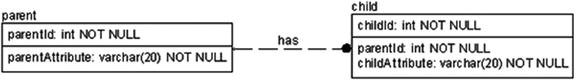
Figure 6-30. Required parent-to-child relationship requires NOT NULL on the migrated key
This is all you need to do, because SQL Server knows that when the referencing key allows a NULL, the relationship value is optional. In our model, represented in Figure 6-31, we have seven relationships modeled.

Figure 6-31. Messaging model for reference
Recall from Figure 6-9 that we had given the relationships a verb phrase, which is used to read the name. For example, in the relationship between User and Message, we have two relationships. One of them was verb phrased as "Is Sent" as in User-Is Sent-Message. In order to get interesting usage of these verb phrases, I will use them as part of the name of the constraint, so that constraint will be named:
FKMessagingUser$IsSent$Messages_Message
Doing this greatly improves the value of the names for constraints, particularly when you have more than one foreign key going between the same two tables. Now, let’s go through the seven constraints and decide the type of options to use on the foreign key relationships. First up is the relationship between AttendeeType and MessagingUser. Since it uses a natural key, it is a target for the UPDATE CASCADE option. However, note that if you have a lot of MessagingUser rows, this operation can be very costly, so it should be done during off-hours. And, if it turns out it is done very often, the choice to use a volatile natural key value ought to be reconsidered. We will use ON DELETE NO ACTION, because we don’t usually want to cascade a delete from a table that is strictly there to implement a domain.
ALTER TABLE Attendees.MessagingUser
       ADD CONSTRAINT FKMessagingUser$IsSent$Messages_Message
            FOREIGN KEY (AttendeeType) REFERENCES Attendees.AttendeeType(AttendeeType)
            ON UPDATE CASCADE
            ON DELETE NO ACTION;
Next, let’s consider the two relationships between the MessagingUser table and the UserConnection table. Since we modeled both of the relationships as required, if one user is deleted (as opposed to being disabled), then we would delete all connections to and from the MessagingUser table. Hence, you might consider implementing both of these as DELETE CASCADE. However, if you execute the following statements:
ALTER TABLE Attendees.UserConnection
        ADD CONSTRAINT
          FKMessagingUser$ConnectsToUserVia$Attendees_UserConnection
        FOREIGN KEY (MessagingUserId) REFERENCES Attendees.MessagingUser(MessagingUserId)
        ON UPDATE NO ACTION
        ON DELETE CASCADE;
ALTER TABLE Attendees.UserConnection
        ADD CONSTRAINT
          FKMessagingUser$IsConnectedToUserVia$Attendees_UserConnection
        FOREIGN KEY  (ConnectedToMessagingUserId)
                              REFERENCES Attendees.MessagingUser(MessagingUserId)
        ON UPDATE NO ACTION
        ON DELETE CASCADE;
Introducing FOREIGN KEY constraint ’FKMessagingUser$IsConnectedToUserVia$Attendees_UserConnection’ on table ’UserConnection’ may cause cycles or multiple cascade paths. Specify ON DELETE NO ACTION or ON UPDATE NO ACTION, or modify other FOREIGN KEY constraints.
Basically, this message is stating that you cannot have two CASCADE operations on the same table. This even more limits the value of the CASCADE operations. Instead, we will use NO ACTION for the DELETE and will just have to implement the cascade in the client code or using a trigger (which I will do as an example).
I will also note that, in many ways, having these limitations on cascading operations is probably a good thing. Too much automatically executing code is going to make developers antsy about what is going on with the data, and if you accidentally delete a user, having NO ACTION specified can actually be a good thing to stop dumb mistakes.
I will change the constraints to NO ACTION and re-create (dropping the one that was created first):
ALTER TABLE Attendees.UserConnection
        DROP CONSTRAINT
          FKMessagingUser$ConnectsToUserVia$Attendees_UserConnection;
GO
ALTER TABLE Attendees.UserConnection
        ADD CONSTRAINT
          FKMessagingUser$ConnectsToUserVia$Attendees_UserConnection
        FOREIGN KEY (MessagingUserId) REFERENCES Attendees.MessagingUser(MessagingUserId)
        ON UPDATE NO ACTION
        ON DELETE NO ACTION;
ALTER TABLE Attendees.UserConnection
        ADD CONSTRAINT
          FKMessagingUser$IsConnectedToUserVia$Attendees_UserConnection
        FOREIGN KEY  (ConnectedToMessagingUserId)
                              REFERENCES Attendees.MessagingUser(MessagingUserId)
        ON UPDATE NO ACTION
        ON DELETE NO ACTION;
GO
And the following INSTEAD OF trigger will go ahead and delete the rows before the actual operation that the user tried is executed:
CREATE TRIGGER MessagingUser$InsteadOfDeleteTrigger
ON Attendees.MessagingUser
INSTEAD OF DELETE AS
BEGIN
   DECLARE @msg varchar(2000),    --used to hold the error message
   --use inserted for insert or update trigger, deleted for update or delete trigger
   --count instead of @@rowcount due to merge behavior that sets @@rowcount to a number
   --that is equal to number of merged rows, not rows being checked in trigger
           @rowsAffected int = (select count(*) from inserted);
           @rowsAffected int = (select count(*) from deleted);
   --no need to continue on if no rows affected
   IF @rowsAffected = 0 RETURN;
   SET NOCOUNT ON; --to avoid the rowcount messages
   SET ROWCOUNT 0; --in case the client has modified the rowcount
   BEGIN TRY
          --[validation section]
          --[modification section]
          --implement multi-path cascade delete in trigger
          DELETE FROM Attendees.UserConnection
          WHERE  MessagingUserId IN (SELECT MessagingUserId FROM DELETED);
          DELETE FROM Attendees.UserConnection
          WHERE  ConnectedToMessagingUserId IN (SELECT MessagingUserId FROM DELETED);
          --<perform action>
          DELETE FROM Attendees.MessagingUser
          WHERE  MessagingUserId IN (SELECT MessagingUserId FROM DELETED);
   END TRY
   BEGIN CATCH
          IF @@trancount > 0
              ROLLBACK TRANSACTION;
          THROW;
     END CATCH;
END;
For the two relationships between MessagingUser and Message, it may seem like we want to use cascade operations, but in this case, since we implemented a disabled indicator in the MessagingUser table, we would probably not use cascade operations. If the MessagingUser had not created message rows yet, it could be deleted, otherwise it would usually be disabled (and the row would not be deleted, which would cause the previous trigger to fail and leave the connection rows alone too).
If a system administrator wants to remove the user completely, a module would likely be created to manage this operation, as it would be the exception rather than the rule. So for this example, we will implement NO ACTION on DELETE:
ALTER TABLE Messages.Message
        ADD CONSTRAINT FKMessagingUser$Sends$Messages_Message FOREIGN KEY
            (MessagingUserId) REFERENCES Attendees.MessagingUser(MessagingUserId)
        ON UPDATE NO ACTION
        ON DELETE NO ACTION;
ALTER TABLE Messages.Message
        ADD CONSTRAINT FKMessagingUser$IsSent$Messages FOREIGN KEY
            (SentToMessagingUserId) REFERENCES Attendees.MessagingUser(MessagingUserId)
        ON UPDATE NO ACTION
        ON DELETE NO ACTION;
Whether to use cascading operations should not be considered lightly. NO ACTION relationships prevent mistakes from causing calamity. CASCADE operations (including SET NULL and SET DEFAULT, which give you additional possibilities for controlling cascading operations), are powerful tools to make coding easier, but could wipe out a lot of data. For example, if you case cascade from MessagingUser to Message and UserConnection, then do DELETE MessagingUser, data can be gone in a hurry.
The next relationship we will deal with is between Topic and MessageTopic. We don’t want Topics to be deleted once set up and used, other than by the administrator as a special operation perhaps, where special requirements are drawn up and not done as a normal thing. Hence, we use the DELETE NO ACTION:
ALTER TABLE Messages.MessageTopic
        ADD CONSTRAINT
           FKTopic$CategorizesMessagesVia$Messages_MessageTopic FOREIGN KEY
             (TopicId) REFERENCES Messages.Topic(TopicId)
        ON UPDATE NO ACTION
        ON DELETE NO ACTION;
The next-to-last relationship to implement is the MessageTopic to Message relationship. Just like the Topic to MessageTopic relationship, there is no need to automatically delete messages if the topic is deleted.
ALTER TABLE Messages.MessageTopic
        ADD CONSTRAINT FKMessage$isCategorizedVia$MessageTopic FOREIGN KEY
            (MessageId) REFERENCES Messages.Message(MessageId)
        ON UPDATE NO ACTION
        ON DELETE NO ACTION;
One of the primary limitations on constraint-based foreign keys is that the tables participating in the relationship cannot span different databases (or different engine models, in that a memory-optimized table’s foreign keys cannot reference an on-disk table’s constraints). When this situation occurs, these relationship types need to be implemented via triggers from the on-disk table, or interpreted T-SQL stored procedures for in-memory tables.
While cross-container (as the memory-optimized and on-disk storage/transaction engines are commonly referred to) relationships may be useful at times (more on this in later chapters), it is definitely considered a bad idea to design databases with cross-database relationships. A database should be considered a unit of related tables that are always kept in sync. When designing solutions that extend over different databases or even servers, carefully consider how spreading around references to data that isn’t within the scope of the database will affect your solution. You need to understand that SQL Server cannot guarantee the existence of the value, because SQL Server uses databases as its “container,” and another user could restore a database with improper values, even an empty database, and the cross-database RI would be invalidated. Of course, as is almost always the case with anything that isn’t best-practice material, there are times when cross-database relationships are unavoidable, and I’ll demonstrate building triggers to support this need in the next chapter on data protection.
In the security chapter (Chapter 9), we will discuss more about how to secure cross-database access, but it is generally considered a less than optimal usage. In SQL Server 2012, the concepts of contained databases, and even SQL Azure, the ability to cross database boundaries is changing in ways that will generally be helpful for building secure databases that exist on the same server.
Adding Basic CHECK Constraints
In our database, we have specified a couple of domains that need to be implemented a bit more strictly. In most cases, we can implement validation routines using simple CHECK constraints. CHECK constraints are simple, single-row predicates that can be used to validate the data in a row. The basic syntax is
ALTER TABLE <tableName> [WITH CHECK | WITH NOCHECK]
   ADD [CONSTRAINT <constraintName>]
   CHECK <BooleanExpression>
One thing interesting about CHECK constraints is how the <BooleanExpression> is evaluated. The <BooleanExpression> component is similar to the WHERE clause of a typical SELECT statement, but with the caveat that no subqueries are allowed. (Subqueries are allowed in standard SQL but not in T-SQL. In T-SQL, you must use a function to access other tables.)
CHECK constraints can reference system and user-defined functions and use the name or names of any columns in the table. However, they cannot access any other table, and they cannot access any row other than the current row being modified (except through a function, and the row values you will be checking will already exist in the table). If multiple rows are modified, each row is checked against this expression individually.
The interesting thing about this expression is that, unlike a WHERE clause, the condition is checked for falseness rather than truth. If the result of a comparison is UNKNOWN because of a NULL comparison, the row will pass the CHECK constraint and be entered. Even if this isn’t immediately confusing, it is often confusing when figuring out why an operation on a row did or did not work as you might have expected. For example, consider the Boolean expression value <> ’fred’. If value is NULL, this is accepted, because NULL <> ’fred’ evaluates to UNKNOWN. If value is ’fred’, it fails because ’fred’ <> ’fred’ is False. The reason for the way CHECK constraints work with Booleans is that if the column is defined as NULL, it is assumed that you wish to allow a NULL value for the column value. You can look for NULL values bvy explicitly checking for them using IS NULL or IS NOT NULL. This is useful when you want to ensure that a column that technically allows nulls does not allow NULLs if another column has a given value. As an example, if you have a column defined name varchar(10) null, having a CHECK constraint that says name = ’fred’ technically says name = ’fred’ or name is null. If you want to ensure it is not null if the column NameIsNotNullFlag = 1, you would state ((NameIsNotNullFlag = 1 and Name is not null) or (NameIsNotNullFlag = 0)).
Note that the [WITH CHECK | WITH NOCHECK] specification works just like it did for FOREIGN KEY constraints
In our model, we had two domain predicates specified in the text that we will implement here. The first is the TopicName, which called for us to make sure that the value is not an empty string or all space characters. I repeat it here in Table 6-8 for review.
Table 6-8. Domain: TopicName
|
Property |
Setting |
|---|---|
|
Name |
TopicName |
|
Optional |
No |
|
Datatype |
Unicode text, 30 characters |
|
Value Limitations |
Must not be an empty string or only space characters |
|
Default Value |
n/a |
The maximum length of 30 characters was handled by the datatype of nvarchar(30) we used but now will implement the rest of the value limitations. The method I will use for this is to do an LTRIM on the value and then check the length. If it is 0, it is either all spaces or empty. We used the TopicName domain for two columns, the Name column from Messages.Topic, and the UserDefinedTopicName column from the Messages.MessageTopic table: