
![]()
Index Structures and Application
In this life, we have to make many choices. Some are very important choices. Some are not. Many of our choices are between good and evil. The choices we make, however, determine to a large extent our happiness or our unhappiness, because we have to live with the consequences of our choices.
— James E. Faust, American religious leader, lawyer, and politician
To me, the true beauty of the relational database engine comes from its declarative nature. As a programmer, I simply ask the engine a question, and it answers it. The questions I ask are usually pretty simple; just give me some data from a few tables, correlate it based on a column or two, do a little math perhaps, and give me back information (and naturally do it incredibly fast, if you don’t mind). While simple isn’t always the case, the engine usually obliges with an answer extremely quickly. Usually, but not always. This is where the DBA and data programmers must figure out what the optimizer is doing and help it along. If you are not a technical person, you probably think of query tuning as magic. It is not. What it is is a lot of complex code implementing a massive amount of extremely complex algorithms that allow the engine to answer your questions in a timely manner. With every passing version of SQL Server, that code gets better at turning your request into a set of operations that gives you the answers you desire in remarkably small amounts of time. These operations will be shown to you on a query plan, which is a blueprint of the algorithms used to execute your query. I will use query plans in this chapter to show you how your design choices can affect the way work gets done.
Our part in the process of getting back lightning-fast answers to complex questions is to assist the query optimizer (which takes your query and turns it into a plan of how to run the query), the query processor (which takes the plan and uses it to do the actual work), and the storage engine (which manages IO for the whole process). We do this first by designing and implementing as close to the relational model as possible by normalizing our structures, using good set-based code (no cursors), following best practices with coding T-SQL, and so on. This is obviously a design book, so I won’t cover T-SQL coding, but it is a skill you should master. Consider Apress’s Beginning T-SQL, Third Edition, by Kathi Kellenberger (Aunt Kathi!) and Scott Shaw, or perhaps one of Itzik Ben-Gan’s Inside SQL books on T-SQL, for some deep learning on the subject. Once we have built our systems correctly, the next step is to help out by adjusting the physical structures using proper hardware laid out well on disk subsystems, filegroups, files, partitioning, and configuring our hardware to work best with SQL Server, and with the load we will be, are, and have been placing on the server. This is yet another book’s worth of information, for which I will direct you to a book I recently reviewed as a technical editor, Peter Carter’s Pro SQL Server Administration (Apress, 2015).
In this chapter we are going to focus primarily on the structures that you will be adding and subtracting regularly: indexes. Indexing is a constant balance of helping performance versus harming performance. If you don’t use indexes enough, queries will be slow, as the query processor could have to read every row of every table for every query (which, even if it seems fast on your machine, can cause the concurrency issues we will cover in Chapter 11 by forcing the query processor to lock a lot more memory than is necessary). Use too many indexes, and modifying data could take too long, as indexes have to be maintained. Balance is the key, kind of like matching the amount of fluid to the size of the glass so that you will never have to answer that annoying question about a glass that has half as much fluid as it can hold. (The answer is either that the glass is too large or the server needs to refill your glass immediately, depending on the situation.)
All plans that I present will be obtained using the SET SHOWPLAN_TEXT ON statement. When you’re doing this locally, it is almost always easier to use the graphical showplan from Management Studio. However, when you need to post the plan or include it in a document, use one of the SET SHOWPLAN_TEXT commands. You can read about this more in SQL Server Books Online. Note that using SET SHOWPLAN_TEXT (or the other versions of SET SHOWPLAN that are available, such as SET SHOWPLAN_XML) commands does not actually execute the statement/batch; rather, they show the estimated plan. If you need to execute the statement (like to get some dynamic SQL statements to execute to see the plan), you can use SET STATISTICS PROFILE ON to get the plan and some other pertinent information about what has been executed. Each of these session settings will need to be turned OFF explicitly once you have finished, or they will continue executing returning plans where you don’t want so.
Everything we have done so far has been centered on the idea that the quality of the data is the number one concern. Although this is still true, in this chapter, we are going to assume that we’ve done our job in the logical and implementation phases, so the data quality is covered. Slow and right is always better than fast and wrong (how would you like to get paid a week early, but only get half your money?), but the obvious goal of building a computer system is to do things right and fast. Everything we do for performance should affect only the performance of the system, not the data quality in any way.
We have technically added indexes in previous chapters, as a side effect of adding primary key and unique constraints (in that a unique index is built by SQL Server to implement the uniqueness condition). In many cases, those indexes will turn out to be almost all of what you need to make normal OLTP queries run nicely, since the most common searches that people will do will be on identifying information.
What complicates all of our choices at this point in the process in the fifth edition of this book is that Microsoft has added an additional engine to the mix, in both the box and cloud versions of the product. I have noted in Chapters 6 and onward that these different versions exist, and that some of the sample code from those chapters will have downloaded versions to show how it might be coded with the different engines. But the differences are more than code. The design of the logical database isn’t that much different, and what is put into the physical database needn’t change considerably either. But there are internal differences to how indexes work that will change some of the implementation, which I will explore in this chapter. Chapter 11 will discuss how these changes affect concurrency and isolation, and finally, Chapter 13 will discuss changes in coding you will see. For now, we will start with the more common on-disk indexes, and then we will look at the memory-optimized index technologies, including indexes on in-memory OLTP table and columnstore indexes (which will be discussed in more detail in Chapter 14 as well).
Indexing Overview
Indexes allow the SQL Server engine to perform fast, targeted data retrieval rather than simply scanning though the entire table. A well-placed index can speed up data retrieval by orders of magnitude, while a haphazard approach to indexing can actually have the opposite effect when creating, updating, or deleting data.
Indexing your data effectively requires a sound knowledge of how that data will change over time, the sort of questions that will be asked of it, and the volume of data that you expect to be dealing with. Unfortunately, this is what makes any topic about physical tuning so challenging. To index effectively, you almost need the psychic ability to foretell the future of your exact data usage patterns. Nothing in life is free, and the creation and maintenance of indexes can be costly. When deciding to (or not to) use an index to improve the performance of one query, you have to consider the effect on the overall performance of the system.
In the upcoming sections, I’ll do the following:
- Introduce the basic structure of an index.
- Discuss the two fundamental types of indexes and how their structure determines the structure of the table.
- Demonstrate basic index usage, introducing you to the basic syntax and usage of indexes.
- Show you how to determine whether SQL Server is likely to use your index and how to see if SQL Server has used your index.
If you are producing a product for sale that uses SQL Server as the backend, indexes are truly going to be something that you could let your customers manage (unless you can truly effectively constrain how users will use your product). For example, if you sell a product that manages customers, and your basic expectation is that they will have around 1,000 customers, what happens if one wants to use it with 100,000 customers? Do you not take their money? Of course you do, but what about performance? Hardware improvements generally cannot even give linear improvement in performance. So if you get hardware that is 100 times “faster,” you would be extremely fortunate to get close to 100 times improvement. However, adding a simple index can provide 100,000 times improvement that may not even make a difference at all on the smaller data set. (This is not to pooh-pooh the value of faster hardware at all. The point is that, situationally, you get far greater gain from writing better code than you do from just throwing hardware at the problem. The ideal situation is adequate hardware and excellent code, naturally.)
Basic Index Structure
An index is a structure that SQL Server can maintain to optimize access to the physical data in a table. An index can be on one or more columns of a table. In essence, an index in SQL Server works on the same principle as the index of a book. It organizes the data from the column (or columns) of data in a manner that’s conducive to fast, efficient searching, so you can find a row or set of rows without looking at the entire table. It provides a means to jump quickly to a specific piece of data, rather than just starting on page one each time you search the table and scanning through until you find what you’re looking for. Even worse, when you are looking for one specific row (and you know that the value you are searching for is unique), unless SQL Server knows exactly how many rows it is looking for, it has no way to know if it can stop scanning data when one row had been found.
As an example, consider that you have a completely unordered list of employees and their details in a book. If you had to search this list for persons named ’Davidson’, you would have to look at every single name on every single page. Soon after trying this, you would immediately start trying to devise some better manner of searching. On first pass, you would probably sort the list alphabetically. But what happens if you needed to search for an employee by an employee identification number? Well, you would spend a bunch of time searching through the list sorted by last name for the employee number. Eventually, you could create a list of last names and the pages you could find them on and another list with the employee numbers and their pages. Following this pattern, you would build indexes for any other type of search you’d regularly perform on the list. Of course, SQL Server can page through the phone book one name at a time in such a manner that, if you need to do it occasionally, it isn’t such a bad thing, but looking at two or three names per search is always more efficient than two or three hundred, much less two or three million.
Now, consider this in terms of a table like an Employee table. You might execute a query such as the following:
SELECT LastName, <EmployeeDetails>
FROM Employee
WHERE LastName = ’Davidson’;
In the absence of an index to rapidly search, SQL Server will perform a scan of the data in the entire table (referred to as a table scan) on the Employee table, looking for rows that satisfy the query predicate. A full table scan generally won’t cause you too many problems with small tables, but it can cause poor performance for large tables with many pages of data, much as it would if you had to manually look through 20 values versus 2,000. Of course, on your development box, you probably won’t be able to discern the difference between a seek and a scan (or even hundreds of scans). Only when you are experiencing a reasonably heavy load will the difference be noticed. (And as we will notice in the next chapter, the more rows SQL Server needs to touch, the more blocking you may do to other users.)
If we instead created an index on the LastName column, the index creates a structure to allow searching for the rows with the matching LastName in a logical fashion and the database engine can move directly to rows where the last name is Davidson and retrieve the required data quickly and efficiently. And even if there are ten people with the last name of ’Davidson’, SQL Server knows to stop when it hits ’Davidtown’.
Of course, as you might imagine, the engineer types who invented the concept of indexing and searching data structures don’t simply make lists to search through. Instead, most indexes are implemented using what is known as a balanced tree (B-tree) structure (some others are built using hash structures, as we cover when we get to the in-memory OLTP section, but B-trees will be overwhelmingly the norm, so they get the introduction). The B-tree index is made up of index pages structured, again, much like an index of a book or a phone book. Each index page contains the first value in a range and a pointer to the next lower page in the index. The pages on last level in the index are referred to as the leaf pages, which contain the actual data values that are being indexed, plus either the data for the row or pointers to the data. This allows the query processor to go directly to the data it is searching for by checking only a few pages, even when there are millions of values in the index.
Figure 10-1 shows an example of the type of B-tree that SQL Server uses for on-disk indexes (memory-optimized indexes are different and will be covered later). Each of the outer rectangles is an 8K index page, just as we discussed earlier. The three values—’A, ’J’, and ’P’—are the index keys in this top-level page of the index. The index page has as many index keys as will fit physically on the page. To decide which path to follow to reach the lower level of the index, we have to decide if the value requested is between two of the keys: ’A’ to ’I’, ’J’ to ’P’, or greater than ’P’. For example, say the value we want to find in the index happens to be ’I’. We go to the first page in the index. The database determines that ’I’ doesn’t come after ’J’, so it follows the ’A’ pointer to the next index page. Here, it determines that ’I’ comes after ’C’ and ’G’, so it follows the ’G’ pointer to the leaf page.

Figure 10-1. Basic index structure
Each of these pages is 8KB in size. Depending on the size of the key (determined by summing the data lengths of the columns in the key, up to a maximum of 1,700 bytes for some types of indexes), it’s possible to have anywhere from 4 entries to over 1,000 on a single page. The more keys you can fit onto a single index page, allows that page to support that many more children index pages. Therefore a given level of the index B-Tree can support more index pages. The more pages are linked from each level to the next, and finally, the fewer numbers of steps from the top page of the index to reach the leaf.
B-tree indexes are extremely efficient, because for an index that stores only 500 different values on a page—a reasonable number for a typical index of an integer—it has 500 pointers to the next level in the index, and the second level has 500 pages with 500 values each. That makes 250,000 different pointers on that level, and the next level has up to 250,000 × 500 pointers. That’s 125,000,000 different values in just a three-level index. Change that to a 100-byte key, do the math, and you will see why smaller keys (like an integer, which is just 4 bytes) are better! Obviously, there’s overhead to each index key, and this is just a rough estimation of the number of levels in the index.
Another idea that’s mentioned occasionally is how well balanced the tree is. If the tree is perfectly balanced, every index page would have exactly the same number of keys on it. Once the index has lots of data on one end, or data gets moved around on it for insertions or deletions, the tree becomes ragged, with one end having one level, and another many levels. This is why you have to do some basic maintenance on the indexes, something I have mentioned already.
This is just a general overview of what an index is, and there are several variations of types of indexes in use with SQL Server. Many use a B-Tree structure for their basis, but some use hashing, and others use columnar structures. The most important aspect to understand at this point? Indexes speed access to rows by giving you quicker access to some part of the table so that you don’t have to look at every single row and inspect it individually.
On-Disk Indexes
To understand indexes on on-disk objects, it helps to have a working knowledge of the physical structures of a database. At a high level, the storage component of the on-disk engine works with a hierarchy of structures, starting with the database, which is broken down into filegroups (with one PRIMARY filegroup always existing), and each filegroup containing a number of files. As we discussed in Chapter 8, a filegroup can contain files for filestream, which in-memory OLTP also uses; but we are going to keep this simple and just talk about simple files that store basic data. This is shown in Figure 10-2.

Figure 10-2. Generalized database and filegroup structure
You control the placement of objects that store physical data pages at the filegroup level (code and metadata is always stored on the primary filegroup, along with all the system objects). New objects created are placed in the default filegroup, which is the PRIMARY filegroup (every database has one as part of the CREATE DATABASE statement, or the first file specified is set to primary) unless another filegroup is specified in any CREATE <object> commands. For example, to place an object in a filegroup other than the default, you need to specify the name of the filegroup using the ON clause of the table- or index-creation statement:
CREATE TABLE <tableName>
(...)  ON <fileGroupName>
This command assigns the table to the filegroup, but not to any particular file. There are commands to place indexes and constraints that are backed with unique indexes on a different filegroup as well. An important part of tuning can be to see if there is any pressure on your disk subsystems and, if so, possibly redistribute data to different disks using filegroups. If you want to see what files you have in your database, you can query the sys.filegroups catalog view:
USE <databaseName>;
GO
SELECT CASE WHEN fg.name IS NULL
                 --other, such as logs
                 THEN CONCAT(’OTHER-’,df.type_desc COLLATE database_default)
                        ELSE fg.name END AS file_group,
       df.name AS file_logical_name,
       df.physical_name AS physical_file_name
FROM   sys.filegroups AS fg
         RIGHT JOIN sys.database_files AS df
            ON fg.data_space_id = df.data_space_id;
As shown in Figure 10-3, files are further broken down into a number of extents, each consisting of eight separate 8KB pages where tables, indexes, and so on are physically stored. SQL Server only allocates space in a database in uniques of extents. When files grow, you will notice that the size of files will be incremented only in 64KB increments.

Figure 10-3. Files and extents
Each extent in turn has eight pages that hold one specific type of data each:
- Data: Table data.
- Index: Index data.
- Overflow data: Used when a row is greater than 8,060 bytes or for varchar(max), varbinary(max), text, or image values.
- Allocation map: Information about the allocation of extents.
- Page free space: Information about what different pages are allocated for.
- Index allocation: Information about extents used for table or index data.
- Bulk changed map: Extents modified by a bulk INSERT operation.
- Differential changed map: Extents that have changed since the last database backup command. This is used to support differential backups.
In larger databases, most extents will contain just one type of page, but in smaller databases, SQL Server can place any kind of page in the same extent. When all data is of the same type, it’s known as a uniform extent. When pages are of various types, it’s referred to as a mixed extent.
SQL Server places all on-disk table data in pages, with a header that contains metadata about the page (object ID of the owner, type of page, and so on), as well as the rows of data, which is what we typically care about as programmers.
Figure 10-4 shows a typical data page from a table. The header of the page contains identification values such as the page number, the object ID of the object the data is for, compression information, and so on. The data rows hold the actual data. Finally, there’s an allocation block that has the offsets/pointers to the row data.

Figure 10-4. Data pages
Figure 10-4 also shows that there are pointers from the next to the previous rows. These pointers are added when pages are ordered, such as in the pages of an index. Heap objects (tables with no clustered index) are not ordered. I will cover this in the next two sections.
The other kind of page that is frequently used that you need to understand is the overflow page. It is used to hold row data that won’t fit on the basic 8,060-byte page. There are two reasons an overflow page is used:
- The combined length of all data in a row grows beyond 8,060 bytes. In this case, data goes on an overflow page automatically, allowing you to have virtually unlimited row sizes (with the obvious performance concerns that go along with that, naturally).
- By setting the sp_tableoption setting on a table for large value types out of row to 1, all the (max) and XML datatype values are immediately stored out of row on an overflow page. If you set it to 0, SQL Server tries to place all data on the main page in the row structure, as long as it fits into the 8,060-byte row. The default is 0, because this is typically the best setting when the typical values are short enough to fit on a single page.
For example, Figure 10-5 depicts the type of situation that might occur for a table that has the large value types out of row set to 1. Here, Data Row 1 has two pointers to support two varbinary(max) columns: one that spans two pages and another that spans only a single page. Using all of the data in Data Row 1 will now require up to four reads (depending on where the actual page gets stored in the physical structures), making data access far slower than if all of the data were on a single page. This kind of performance problem can be easy to overlook, but on occasion, overflow pages will really drag down your performance, especially when other programmers use SELECT * on tables where they don’t really need all of the data.

Figure 10-5. Sample overflow pages
The overflow pages are linked lists that can accommodate up to 2GB of storage in a single column. Generally speaking, it isn’t really a very good idea to store 2GB in a single column (or even a row), but the ability to do so is available if needed.
Storing large values that are placed off of the main page will be far costlier when you need these values than if all of the data can be placed in the same data page. On the other hand, if you seldom use the data in your queries, placing them off the page can give you a much smaller footprint for the important data, requiring far less disk access on average. It is a balance that you need to take care with, as you can imagine how costly a table scan of columns that are on the overflow pages is going to be. Not only will you have to read extra pages, you’ll have to be redirected to the overflow page for every row that’s overflowed.
When you get down to the row level, the data is laid out with metadata, fixed length fields, and variable length fields, as shown in Figure 10-6. (Note that this is a generalization, and the storage engine does a lot of stuff to the data for optimization, especially when you enable compression.)

Figure 10-6. Data row
The metadata describes the row, gives information about the variable length fields, and so on. Generally speaking, since data is dealt with by the query processor at the page level, even if only a single row is needed, data can be accessed very rapidly no matter the exact physical representation.
The maximum amount of data that can be placed on a single page (including overhead from variable fields) is 8,060 bytes. As illustrated in Figure 10-5, when a data row grows larger than 8,060 bytes, the data in variable length columns can spill out onto an overflow page. A 16-byte pointer is left on the original page and points to the page where the overflow data is placed.
One last concept we need to discuss, and that is page splits. When inserting or updating rows, SQL Server might have to rearrange the data on the pages due to the pages being filled up. Such rearranging can be a particularly costly operation. Consider the situation from our example shown in Figure 10-7, assuming that only three values can fit on a page.

Figure 10-7. Sample data page before page split
Say we want to add the value Bear to the page. If that value won’t fit onto the page, the page will need to be reorganized. Pages that need to be split are split into two, generally with 50% of the data on one page, and 50% on the other (there are usually more than three values on a real page). Once the page is split and its values are reinserted, the new pages would end up looking something like Figure 10-8.

Figure 10-8. Sample data page after page split
Page splits are costly operations and can be terrible for performance, because after the page split, data won’t be located on successive physical pages. This condition is commonly known as fragmentation. Page splits occur in a normal system and are simply a part of adding data to your table. However, they can occur extremely rapidly and seriously degrade performance if you are not careful. Understanding the effect that page splits can have on your data and indexes is important as you tune performance on tables that have large numbers of inserts or updates.
To tune your tables and indexes to help minimize page splits, you can use the FILL FACTOR of the index. When you build or rebuild an index or a table (using ALTER TABLE <tablename> REBUILD, a command that was new in SQL Server 2008), the fill factor indicates how much space is left on each page for future data. If you are inserting random values all over the structures, a common situation that occurs when you use a nonsequential uniqueidentifier for a primary key, you will want to leave adequate space on each page to cover the expected number of rows that will be created in the future. During a page split, the data page is always split approximately fifty-fifty, and it is left half empty on each page, and even worse, the structure is becoming, as mentioned, fragmented.
Now that we have looked at the basic physical structures, let’s get down to the index structures that we will commonly work with. There are two different types of indexes:
- Clustered: This type orders the physical table in the order of the index.
- Nonclustered: These are completely separate structures that simply speed access.
How indexes are structured internally is based on the existence (or nonexistence) of a clustered index. For the nonleaf pages of an index, everything is the same for all indexes. However, at the leaf node, the indexes get quite different—and the type of index used plays a large part in how the data in a table is physically organized. In the upcoming sections, I’ll discuss how the different types of indexes affect the table structure and which is best in which situation.
The examples in this section on indexes will mostly be based on tables from the WideWorldImporters database you can download from Microsoft in some manner (as I am writing this chapter, it was located on GitHub).
Clustered Indexes
In the following sections, I will discuss the structure of a clustered index, followed by showing the usage patterns and examples of how these indexes are used.
Structure
A clustered index physically orders the pages of the data in the table by making the leaf pages of the index be the data pages of the table. Each of the data pages is then linked to the next page in a doubly linked list to provide ordered scanning. Hence, the records in the physical structure are sorted according to the fields that correspond to the columns used in the index. Tables with a clustered index are referred to as clustered tables.
The key of a clustered index is referred to as the clustering key. For clustered indexes that aren’t defined as unique, each record has a 4-byte value (commonly known as an uniquifier) added to each value in the index where duplicate values exist. For example, if the values were A, B, and C, you would be fine. But, if you added another value B, the values internally would be A, B + 4ByteValue, B + Different4ByteValue, and C. Clearly, it is not optimal to get stuck with 4 bytes on top of the other value you are dealing with in every level of the index, so in general, you should try to define the key columns of the clustered index on column(s) where the values are unique, and the smaller the better, as the clustering key will be employed in every other index that you place on a table that has a clustered index.
Figure 10-9 shows, at a high level, what a clustered index might look like for a table of animal names. (Note that this is just a partial example; there would likely be more second-level pages for Horse and Python at a minimum.)

Figure 10-9. Clustered index example
You can have only one clustered index on a table, because the table cannot be ordered on more than one set of columns. (Remember this; it is one of the most fun interview questions. Answering anything other than “one clustered index per table” leads to a fun line of follow-up questioning.)
A good real-world example of a clustered index would be a set of old-fashioned encyclopedias. Each book is a level of the index, and on each page, there is another level that denotes the things you can find on each page (e.g., Office–Officer). Then each topic is the leaf level of the index. These books are clustered on the topics in the encyclopedia, just as the example is clustered on the name of the animal. In essence, the entire set of books is a table of information in clustered order. And indexes can be partitioned as well. The encyclopedias are partitioned by letter into multiple books.
Now, consider a dictionary. Why are the words sorted, rather than just having a separate index with the words not in order? I presume that at least part of the reason is to let the readers scan through words they don’t know exactly how to spell, checking the definition to see if the word matches what they expect. SQL Server does something like this when you do a search. For example, back in Figure 10-9, if you were looking for a cat named George, you could use the clustered index to find rows where animal = ’Cat’, then scan the data pages for the matching pages for any rows where name = ’George’.
I must caution you that although it’s true, physically speaking, that tables are stored in the order of the clustered index, logically speaking, tables must be thought of as having no order. This lack of order is a fundamental truth of relational programming: you aren’t required to get back data in the same order when you run the same query twice. The ordering of the physical data can be used by the query processor to enhance your performance, but during intermediate processing, the data can be moved around in any manner that results in faster processing the answer to your query. It’s true that you do almost always get the same rows back in the same order, mostly because the optimizer is almost always going to put together the same plan every time the same query is executed under the same conditions. However, load up the server with many requests, and the order of the data might change so SQL Server can best use its resources, regardless of the data’s order in the structures. SQL Server can choose to return data to us in any order that’s fastest for it. If disk drives are busy in part of a table and it can fetch a different part, it will. If order matters, use ORDER BY clauses to make sure that data is returned as you want.
Using the Clustered Index
As mentioned earlier, the clustering key you choose has implications for the rest of your physical design. The column you use for the clustered index will become a part of every index for your table, so it has heavy implications for all indexes. Because of this, for a typical OLTP system, a very common practice is to choose a surrogate key value, often the primary key of the table, since the surrogate can be kept very small.
Using the surrogate key as the clustering key is usually a great decision, not only because it is a small key (most often, the datatype is an integer that requires only 4 bytes or possibly less using compression), but also because it’s always a unique value. As mentioned earlier, a nonunique clustering key has a 4-byte uniquifier tacked onto its value when keys are not unique. It also helps the optimizer that an index has only unique values, because it knows immediately that for an equality operator, either 1 or 0 values will match. Because the surrogate key is often used in joins, it’s helpful to have smaller keys for the primary key.
![]() Caution Using a GUID for a surrogate key is becoming the vogue these days, but be careful. GUIDs are 16 bytes wide, which is a fairly large amount of space, but that is really the least of the problem. GUIDs are random values, in that they generally aren’t monotonically increasing, and a new GUID could sort anywhere in a list of other GUIDs and end up causing large amounts of page splits. The only way to make GUIDs a reasonably acceptable type is to use the NEWSEQUENTIALID() function (or one of your own) to build sequential GUIDS, but it only works with unique identifier columns in a default constraint, and does not guarantee sequential order with existing data after a reboot. Seldom will the person architecting a solution that is based on GUID surrogates want to be tied down to using a default constraint to generate surrogate values. The ability to generate GUIDs from anywhere and ensure their uniqueness is part of the lure of the siren call of the 16-byte value. In SQL Server 2012 and later, the use of the sequence object to generate guaranteed unique values could be used in lieu of GUIDs.
Caution Using a GUID for a surrogate key is becoming the vogue these days, but be careful. GUIDs are 16 bytes wide, which is a fairly large amount of space, but that is really the least of the problem. GUIDs are random values, in that they generally aren’t monotonically increasing, and a new GUID could sort anywhere in a list of other GUIDs and end up causing large amounts of page splits. The only way to make GUIDs a reasonably acceptable type is to use the NEWSEQUENTIALID() function (or one of your own) to build sequential GUIDS, but it only works with unique identifier columns in a default constraint, and does not guarantee sequential order with existing data after a reboot. Seldom will the person architecting a solution that is based on GUID surrogates want to be tied down to using a default constraint to generate surrogate values. The ability to generate GUIDs from anywhere and ensure their uniqueness is part of the lure of the siren call of the 16-byte value. In SQL Server 2012 and later, the use of the sequence object to generate guaranteed unique values could be used in lieu of GUIDs.
The clustered index won’t always be used for the surrogate key or even the primary key. Other possible uses can fall under the following types:
- Range queries: Having all the data in order usually makes sense when there’s data for which you often need to get a range, such as from A to F.
- Data that’s always accessed sequentially: Obviously, if the data needs to be accessed in a given order, having the data already sorted in that order will significantly improve performance.
- Queries that return large result sets: This point will make more sense once I cover nonclustered indexes, but for now, note that having the data on the leaf index page saves overhead.
The choice of how to pick the clustered index depends on several factors, such as how many other indexes will be derived from this index, how big the key for the index will be, and how often the value will change. When a clustered index value changes, every index on the table must also be touched and changed, and if the value can grow larger, well, then we might be talking page splits. This goes back to understanding the users of your data and testing the heck out of the system to verify that your index choices don’t hurt overall performance more than they help. Speeding up one query by using one clustering key could hurt all queries that use the nonclustered indexes, especially if you chose a large key for the clustered index.
Frankly, in an OLTP setting, in all but the most unusual cases, I stick with a surrogate key for my clustering key, usually one of the integer types or sometimes even the unique identifier (GUID) type. I use the surrogate key because so many of the queries you do for modification (the general goal of the OLTP system) will access the data via the primary key. You then just have to optimize retrievals, which should also be of generally small numbers of rows, and doing so is usually pretty easy.
Another thing that is good about using the clustered index on a monotonically increasing value is that page splits over the entire index are greatly decreased. The table grows only on one end of the index, and while it does need to be rebuilt occasionally using ALTER INDEX REORGANIZE or ALTER INDEX REBUILD, you don’t end up with page splits all over the table. You can decide which to do by using the criteria stated by SQL Server Books Online. By looking in the dynamic management view (DMV) sys.dm_db_index_physical_stats, you can use REBUILD on indexes with greater than 30% fragmentation and use REORGANIZE otherwise. Now, let’s look at an example of a clustered index in use. If you select all of the rows in a clustered table, you’ll see a Clustered Index Scan in the plan. For this we will use the Application.Cities table from WideWorldImporters, with the following structure:
CREATE TABLE Application.Cities
(
    CityID int NOT NULL CONSTRAINT PK_Application_Cities PRIMARY KEY CLUSTERED,
    CityName nvarchar(50) NOT NULL,
    StateProvinceID int NOT NULL
        CONSTRAINT FK_Application_Cities_StateProvinceID_Application_StateProvinces
                REFERENCES Application.StateProvinces (StateProvinceID),
    Location geography NULL,
    LatestRecordedPopulation bigint NULL,
    LastEditedBy int NOT NULL,
    ValidFrom datetime2(7) GENERATED ALWAYS AS ROW START NOT NULL,
    ValidTo datetime2(7) GENERATED ALWAYS AS ROW END NOT NULL,
    PERIOD FOR SYSTEM_TIME (ValidFrom, ValidTo)
) ON USERDATA TEXTIMAGE_ON USERDATA
WITH (SYSTEM_VERSIONING = ON (HISTORY_TABLE = Application.Cities_Archive))
This table has temporal extensions added to it, as covered in Chapter 8. In this version of the example database, there is currently also an index on the StateProvince column, which we will use later in the chapter.
CREATE NONCLUSTERED INDEX FK_Application_Cities_StateProvinceID ON Application.Cities
(
        StateProvinceID ASC
)
ON USERDATA;
There are 37,940 rows in the Application.Cities table:
SELECT *
FROM   [Application].[Cities];
The plan for this query is as follows:
    |--Clustered Index Scan
            (OBJECT:([WideWorldImporters].[Application].[Cities].[PK_Application_Cities]))
If you query on a value of the clustered index key, the scan will likely change to a seek, and almost definitely if it is backing the PRIMARY KEY constraint. Although a scan touches all the data pages, a clustered index seek uses the index structure to find a starting place for the scan and knows just how far to scan. For a unique index with an equality operator, a seek would be used to touch one page in each level of the index to find (or not find) a single value on a single data page, for example:
SELECT *
FROM   Application.Cities
WHERE  CityID = 23629; --A favorite city of mine, indeed.
The plan for this query now does a seek:
  |--Clustered Index Seek
           (OBJECT:([WideWorldImporters].[Application].[Cities].[PK_Application_Cities]),
            SEEK:([WideWorldImporters].[Application].[Cities].[CityID]=
                                             CONVERT_IMPLICIT(int,[@1],0)) ORDERED FORWARD)
Note the CONVERT_IMPLICIT of the @1 value. This shows the query is being parameterized for the plan, and the variable is cast to an integer type. In this case, you’re seeking in the clustered index based on the SEEK predicate of CityID = 23629. SQL Server will create a reusable plan by default for simple queries. Any queries that are executed with the same exact format, and a simple integer value would use the same plan. You can let SQL Server parameterize more complex queries as well. (For more information, look up “Simple Parameterization and Forced Parameterization” in Books Online.)
You can eliminate the CONVERT_IMPLICIT by explicitly casting the value in your WHERE as WHERE CityID = CAST(23629 AS int):
  |--Clustered Index Seek
           (OBJECT:([WideWorldImporters].[Application].[Cities].[PK_Application_Cities]),
            SEEK:([WideWorldImporters].[Application].[Cities].[CityID]=[@1])
                                                                           ORDERED FORWARD)
Though this not typically done when it is a complementary literal type in the WHERE clause, it can be an issue when you use noncomplimentary types, like when mixing a Unicode value and non-Unicode value, which we will see later in the chapter. Increasing the complexity, now, we search for two rows:
SELECT *
FROM   Application.Cities
WHERE  CityID IN (23629,334);
And in this case, pretty much the same plan is used, except the seek criteria now has an OR in it:
  |--Clustered Index Seek
           (OBJECT:([WideWorldImporters].[Application].[Cities].[PK_Application_Cities]),
            SEEK:([WideWorldImporters].[Application].[Cities].[CityID]=(334)
                  OR
                  [WideWorldImporters].[Application].[Cities].[CityID]=(23629))
                                                                          ORDERED FORWARD)
Note that it did not create a parameterized plan this time, but a fixed one with literals for 334 and 23629. Also note that this plan will be executed as two separate seek operations. If you turn on SET STATISTICS IO before running the query:
SET STATISTICS IO ON;
GO
SELECT *
FROM   [Application].[Cities]
WHERE  CityID IN (23629,334);
GO
SET STATISTICS IO OFF;
you will see that it did two “scans,” which using STATISTICS IO generally means any operation that probes the table, so a seek or scan would show up the same:
Table ’Cities’. Scan count 2, logical reads 4, physical reads 0, read-ahead reads 0, lob logical reads 0, lob physical reads 0, lob read-ahead reads 0.
But whether any given query uses a seek or scan, or even two seeks, can be a pretty complex question. Why it is so complex will become clearer over the rest of the chapter, and it will become instantly clearer how useful a clustered index seek is in the next section on nonclustered indexes.
Nonclustered Indexes
Nonclustered index structures are fully independent of the underlying table. Where a clustered index is like a dictionary with the index physically linked to the table (since the leaf pages of the index are a part of the table), nonclustered indexes are more like indexes in this book. For on-disk tables, nonclustered indexes are completely separate from the data. Instead of the leaf page having all of the data, they have just the index keys (and included values, there are pointers to go to the data pages much like the index of a book contains page numbers).
Each leaf page in a nonclustered index contains some form of link to the rows on the data page. The link from the index to a data row is known as a row locator. Exactly how the row locator of a nonclustered index is structured is based on whether or not the underlying table has a clustered index.
In this section, I will start with the structure of nonclustered indexes, and then look at how these indexes are used.
Structure
The base B-tree of the nonclustered index is very much the same as the B-tree of the clustered index. The difference will be how you get to the actual data. First we will look at an abstract representation of the nonclustered index and then show the differences between the implementation of a nonclustered index when you do and do not also have a clustered index. At an abstract level, all nonclustered indexes follow the basic form shown in Figure 10-10.

Figure 10-10. Sample nonclustered index
The major difference between the two possibilities comes down to the row locator being different based on whether the underlying table has a clustered index. There are two different types of pointer that will be used:
- Tables with a clustered index: Clustering key
- Tables without a clustered index: Pointer to physical location of the data, commonly referred to as a row identifier (RID)
In the next two sections, I’ll explain these in more detail.
![]() Tip You can place nonclustered indexes on a different filegroup than the data pages to maximize the use of your disk subsystem in parallel. Note that the filegroup you place the indexes on ought to be on a different controller channel than the table; otherwise, it’s likely that there will be minimal or no gain.
Tip You can place nonclustered indexes on a different filegroup than the data pages to maximize the use of your disk subsystem in parallel. Note that the filegroup you place the indexes on ought to be on a different controller channel than the table; otherwise, it’s likely that there will be minimal or no gain.
Nonclustered Index on a Clustered Table
When a clustered index exists on the table, the row locator for the leaf node of any nonclustered index is the clustering key from the clustered index. In Figure 10-11, the structure on the right side represents the clustered index, and the structure on the left represents the nonclustered index. To find a value, you start at the leaf node of the nonclustered index and traverse to the leaf pages. The result of the index traversal is one or more clustering keys, which you then use to traverse the clustered index to reach the data.

Figure 10-11. Nonclustered index on a clustered table
The overhead of the operation I’ve just described is minimal as long as you keep your clustering key optimal and the index maintained. While having to scan two indexes is more work than just having a pointer to the physical location, you have to think of the overall picture. Overall, it’s better than having direct pointers to the table, because only minimal reorganization is required for any modification of the values in the table. Consider if you had to maintain a book index manually. If you used the book page as the way to get to an index value and subsequently had to add a page to the book in the middle, you would have to update all of the page numbers. But if all of the topics were ordered alphabetically, and you just pointed to the topic name, adding a topic would be easy.
The same is true for SQL Server, and the structures can be changed thousands of times a second or more. Since there is very little hardware-based information lingering in the structure when built this way, data movement is easy for the query processor, and maintaining indexes is an easy operation. Early versions of SQL Server always used physical location pointers for indexes, and this led to corruption in our indexes and tables (without a clustering key, it still uses pointers, but in a manner that reduces corruption at the cost of some performance). Let’s face it, the people with better understanding of such things also tell us that when the size of the clustering key is adequately small, this method is remarkably faster overall than having pointers directly to the table.
The primary benefit of the key structure becomes more obvious when we talk about modification operations. Because the clustering key is the same regardless of physical location, only the lowest levels of the clustered index need to know where the physical data is. Add to this that the data is organized sequentially, and the overhead of modifying indexes is significantly lowered, making all of the data modification operations far faster. Of course, this benefit is only true if the clustering key rarely, or never, changes. Therefore, the general suggestion is to make the clustering key a small, nonchanging value, such as an identity column (but the advice section is still a few pages away).
Nonclustered Indexes on a Heap
A heap data structure in computer science is a generally unordered binary tree structure. In SQL Server, when a table does not have a clustered index, the table is physically referred to as a heap. A more practical definition of a heap is “a group of things placed or thrown one on top of the other.” This is a great way to explain what happens in a table when you have no clustered index: SQL Server simply puts every new row on the end of the last page for the table. Once that page is filled up, it puts data on the next page or a new page as needed.
When building a nonclustered index on a heap, the row locator is a pointer to the physical page and row that contains the row. As an example, take the example structure from the previous section with a nonclustered index on the name column of an animal table, represented in Figure 10-12.

Figure 10-12. Nonclustered index on a heap
If you want to find the row where name = ’Dog’, you first find the path through the index from the top-level page to the leaf page. Once you get to the leaf page, you get a pointer to the page that has a row with the value, in this case Page 102, Row 1. This pointer consists of the page location and the record number on the page to find the row values (the pages are numbered from 0, and the offset is numbered from 1). The most important fact about this pointer is that it points directly to the row on the page that has the values you’re looking for. The pointer for a table with a clustered index (a clustered table) is different, and this distinction is important to understand because it affects how well the different types of indexes perform.
To avoid the types of physical corruption issues that, as I mentioned in the previous section, can occur when you are constantly managing pointers and physical locations, heaps use a very simple method of keeping the row pointers from getting corrupted: they never change until you rebuild the table. Instead of reordering pages, or changing pointers if the page must be split, it moves rows to a different page and a forwarding pointer is left to point to the new page where the data is now. So if the row where name = ’Dog’ had moved (for example, perhaps due to a large varchar(3000) column being updated from a data length of 10 to 3,000), you might end up with following situation to extend the number of steps required to pick up the data. In Figure 10-13, a forwarding pointer is illustrated.

Figure 10-13. Forwarding pointer
All existing indexes that have the old pointer simply go to the old page and follow the forwarding pointer on that page to the new location of the data. If you are using heaps, which should be rare, it is important to be careful with your structures to make sure that data should rarely be moved around within a heap. For example, you have to be careful if you’re often updating data to a larger value in a variable length column that’s used as an index key, because it’s possible that a row may be moved to a different page. This adds another step to finding the data and, if the data is moved to a page on a different extent, adds another read to the database. This forwarding pointer is immediately followed when scanning the table, eventually causing possible horrible performance over time if it’s not managed.
Space is typically not reused in the heap without rebuilding the table (either by selecting into another table or by using the ALTER TABLE command with the REBUILD option). In the section “Indexing Dynamic Management View Queries” later in this chapter, I will provide a query that will give you information on the structure of your index, including the count of forwarding pointers in your table.
Using the Nonclustered Index
After you have made the ever-important choice of what to use for the clustered index, all other indexes will be nonclustered. In this section, I will cover some of the choices of how to apply nonclustered indexes in the following areas:
- General considerations
- Composite index considerations
- Nonclustered indexes with clustered tables
- Nonclustered indexes on heaps
In reality, many of the topics in this section pertain to clustered indexes—things such as composite indexes, statistics, uniqueness, etc., for certain. I am covering them here because you will typically make these decisions for nonclustered indexes, and choose the clustered index based on patterns of usage as the PRIMARY KEY, though not always. There is a section in the last major section of the chapter where I will discuss this in more detail.
General Considerations
We generally start to get the feeling that indexes are needed because queries are (or seem) slow. Naturally though, lack of indexes is clearly not the only reason that queries are slow. Here are some of the obvious reasons for slow queries:
- Extra heavy user load
- Hardware load
- Network load
- Poorly designed database
- Concurrency configuration issues (as covered in Chapter 11)
After looking for the existence of the preceding reasons, we can pull out Management Studio and start to look at the plans of the slow queries. Most often, slow queries are apparent because either |--Clustered Index Scan or |--Table Scan shows up in the query plan, and those operations take a large percentage of time to execute. Simple, right? Essentially, it is a true enough statement that index and table scans are time consuming, but unfortunately, that really doesn’t give a full picture of the process. It’s hard to make specific indexing changes before knowing about usage, because the usage pattern will greatly affect these decisions, for example:
- Is a query executed once a day, once an hour, or once a minute?
- Is a background process inserting into a table rapidly? Or perhaps inserts are taking place during off-hours?
Using Extended Events and the dynamic management views, you can watch the usage patterns of the queries that access your database, looking for slowly executing queries, poor plans, and so on. After you do this and you start to understand the usage patterns for your database, you need to use that information to consider where to apply indexes—the final goal being that you use the information you can gather about usage and tailor an index plan to solve the overall picture.
You can’t just throw around indexes to fix individual queries. Nothing comes without a price, and indexes definitely have a cost. You need to consider how indexes help and hurt the different types of operations in different ways:
- SELECT: Indexes can only have a beneficial effect on SELECT queries.
- INSERT: An index can only hurt the process of inserting new data into the table (if usually only slightly). As data is created in the table, there’s a chance that the indexes will have to be modified and reorganized to accommodate the new values.
- UPDATE: An update physically requires two or three steps: find the row(s) and change the row(s), or find the row(s), delete it (them), and reinsert it (them). During the phase of finding the row, the index is beneficial, just as for a SELECT. Whether or not it hurts during the second phase depends on several factors, for example:
- Did the index key value change such that it needs to be moved around to different leaf nodes?
- Will the new value fit on the existing page, or will it require a page split?
- DELETE: The delete requires two steps: to find the row and to remove it. Indexes are beneficial to find the row, but on deletion, you might have to do some reshuffling to accommodate the deleted values from the indexes.
You should also realize that for INSERT, UPDATE, or DELETE operations, if triggers on the table exist (or constraints exist that execute functions that reference tables), indexes will affect those operations in the same ways as in the list. For this reason, I’m going to shy away from any generic advice about what types of columns to index. In practice, there are just too many variables to consider.
![]() Tip Too many people start adding nonclustered indexes without considering the costs. Just be wary that every index you add has to be maintained. Sometimes, a query taking 1 second to execute is OK when getting it down to .1 second might slow down other operations considerably. The real question lies in how often each operation occurs and how much cost you are willing to suffer. The hardest part is keeping your tuning hat off until you can really get a decent profile of all operations that are taking place.
Tip Too many people start adding nonclustered indexes without considering the costs. Just be wary that every index you add has to be maintained. Sometimes, a query taking 1 second to execute is OK when getting it down to .1 second might slow down other operations considerably. The real question lies in how often each operation occurs and how much cost you are willing to suffer. The hardest part is keeping your tuning hat off until you can really get a decent profile of all operations that are taking place.
For a good idea of how your current indexes and/or tables are currently being used, you can query the dynamic management view sys.dm_db_index_usage_stats:
SELECT CONCAT(OBJECT_SCHEMA_NAME(i.object_id),’.’,OBJECT_NAME(i.object_id)) AS object_name
      , CASE WHEN i.is_unique = 1 THEN ’UNIQUE ’ ELSE ’’ END +
                i.TYPE_DESC AS index_type
      , i.name as index_name
      , user_seeks, user_scans, user_lookups,user_updates
FROM  sys.indexes AS i
         LEFT OUTER JOIN sys.dm_db_index_usage_stats AS s
              ON i.object_id = s.object_id
                AND i.index_id = s.index_id
                AND database_id = DB_ID()
WHERE  OBJECTPROPERTY(i.object_id , ’IsUserTable’) = 1
ORDER  BY object_name, index_name;
This query will return the name of each object, an index type, an index name, plus the number of
- User seeks: The number of times the index was used in a seek operation
- User scans: The number of times the index was scanned in answering a query
- User lookups: For clustered indexes, the number of times the index was used to resolve the row locator of a nonclustered index search
- User updates: The number of times the index was changed by a user query
This information is very important when trying to get a feel for which indexes might need to be tuned and especially which ones are not doing their jobs because they are mostly getting updated. A particularly interesting thing to look at in an OLTP system is the user_scans on a clustered index. For example, thinking back to our queries of the Application.Cities table, we only have a clustered index on the PRIMARY KEY column CityID. So if we query
SELECT *
FROM   Application.Cities
WHERE  CityName = ’Nashville’;
the plan will be a scan of the clustered index:
|--Clustered Index Scan
          (OBJECT:([WideWorldImporters].[Application].[Cities].[PK_Application_Cities]),
           WHERE:([WideWorldImporters].[Application].[Cities].[CityName]=(N’Nashvile’));
And you will see the user_scans value increase every time you run this query. This is something we can reconcile by adding a nonclustered index to this column, locating it in the USERDATA filegroup, since that is where other objects were created in the DDL I included earlier:
CREATE INDEX CityName ON Application.Cities(CityName) ON USERDATA;
Of course, there are plenty more settings when creating an index, some we will cover, some we will not. If you need to manage indexes, it certainly is a great idea to read the Books Online topic about CREATE INDEX as a start for more information.
![]() Tip You can create indexes inline with the CREATE TABLE statement starting with SQL Server 2014.
Tip You can create indexes inline with the CREATE TABLE statement starting with SQL Server 2014.
Now check the plan of the query again, and you will see:
|--Nested Loops(Inner Join,
              OUTER REFERENCES:([WideWorldImporters].[Application].[Cities].[CityID]))
       |--Index Seek(OBJECT:([WideWorldImporters].[Application].[Cities].[CityName]),
            SEEK:([WideWorldImporters].[Application].[Cities].[CityName]=N’Nashville’)
                                                                           ORDERED FORWARD)
       |--Clustered Index Seek
             (OBJECT:([WideWorldImporters].[Application].[Cities].[PK_Application_Cities]),
              SEEK:([WideWorldImporters].[Application].[Cities].[CityID]=
               [WideWorldImporters].[Application].[Cities].[CityID])
                                                      LOOKUP ORDERED FORWARD)
This not only is more to format, but it looks like it should be a lot more to execute. However, this plan illustrates nicely the structure of a nonclustered index on a clustered table. The second |-- points at the improvement. To find the row with CityName of Nashville, it seeked in the new index. Once it had the index keys for Nashville rows, it took those and joined them together like two different tables, using a Nested Loops join type. For more information about nested loops and other join operators, check Books Online for “Showplan Logical and Physical Operators Reference.”
Determining Index Usefulness
It might seem at this point that all you need to do is look at the plans of queries, look for the search arguments, and put an index on the columns, then things will improve. There’s a bit of truth to this in a lot of cases, but indexes have to be useful to be used by a query. What if the index of a 418-page book has two entries:
- General Topics 1
- Determining Index Usefulness 417
This means that pages 1–416 cover general topics and pages 417-? are about determining index usefulness. This would be useless to you, unless you needed to know about index usefulness. One thing is for sure: you could determine that the index is generally useless pretty quickly. Another thing we all do with the index of a book to see if the index is useful is to take a value and look it up in the index. If what you’re looking for is in there (or something close), you go to the page and check it out.
SQL Server determines whether or not to use your index in much the same way. It has two specific measurements that it uses to decide if an index is useful: the density of values (sometimes known as the selectivity) and a histogram of a sample of values in the table to check against.
You can see these in detail for indexes by using DBCC SHOW_STATISTICS. Our table is very small, so it doesn’t need stats to decide which to use. Instead, we’ll look at the index we just created:
DBCC SHOW_STATISTICS(’Application.Cities’, ’CityName’) WITH DENSITY_VECTOR;
DBCC SHOW_STATISTICS(’Application.Cities’, ’CityName’) WITH HISTOGRAM;
This returns the following sets (truncated for space). The first tells us the size and density of the keys. The second shows the histogram of where the table was sampled to find representative values.
All density   Average Length Columns
------------- -------------- --------------------------
4.297009E-05  17.17427       CityName
2.635741E-05  21.17427       CityName, CityID
RANGE_HI_KEY           RANGE_ROWS    EQ_ROWS       DISTINCT_RANGE_ROWS  AVG_RANGE_ROWS
---------------------- ------------- ------------- -------------------- --------------
Aaronsburg             0             1             0                    1
Addison                123           11            70                   1.757143
Albany                 157           17            108                  1.453704
Alexandria             90            13            51                   1.764706
Alton                  223           13            122                  1.827869
Andover                173           13            103                  1.679612
.........                    ...           ..            ...                  ........
White Oak              183           10            97                   1.886598
Willard                209           10            134                  1.559701
Winchester             188           18            91                   2.065934
Wolverton              232           1             138                  1.681159
Woodstock              137           12            69                   1.985507
Wynnewood              127           2             75                   1.693333
Zwolle                 240           1             173                  1.387283
I won’t cover the DBCC SHOW_STATISTICS command in great detail, but there are several important things to understand. First, consider the density of each column set. The CityName column is the only column that is actually declared in the index, but note that it includes the density of the index column and the clustering key as well.
All the density is calculated approximately by 1/number of distinct rows, as shown here for the same columns as I just checked the density on:
--Used ISNULL as it is easier if the column can be null
--value you translate to should be impossible for the column
--ProductId is an identity with seed of 1 and increment of 1
--so this should be safe (unless a dba does something weird)
SELECT 1.0/ COUNT(DISTINCT ISNULL(CityName,’NotACity’)) AS density,
            COUNT(DISTINCT ISNULL(CityName,’NotACity’)) AS distinctRowCount,
            1.0/ COUNT(*) AS uniqueDensity,
            COUNT(*) AS allRowCount
FROM   Application.Cities;
This returns the following:
density              distinctRowCount uniqueDensity     allRowCount
-------------------- ---------------- ----------------- -----------
0.000042970092       23272            0.000026357406    37940
You can see that the densities match. (The query’s density is in a numeric type, while the DBCC is using a float, which is why they are formatted differently, but they are the same value!) The smaller the number, the better the index, and the more likely it will be easily chosen for use. There’s no magic number, per se, but this value fits into the calculations of which way is best to execute the query. The actual numbers returned from this query might vary slightly from the DBCC value, as a sampled number might be used for the distinct count.
The second thing to understand in the DBCC SHOW_STATISTICS output is the histogram. Even if the density of the index isn’t low, SQL Server can check a given value (or set of values) in the histogram to see how many rows will likely be returned. SQL Server keeps statistics about columns in a table as well as in indexes, so it can make informed decisions as to how to employ indexes or table columns. For example, consider the following rows from the histogram (I have faked some of these results for demonstration purposes):
RANGE_HI_KEY RANGE_ROWS    EQ_ROWS       DISTINCT_RANGE_ROWS  AVG_RANGE_ROWS
------------ ------------- ------------- -------------------- --------------
Aaronsburg   111           58            2                    55.5
Addison      117           67            2                    58.5
...          ...           ...           ...                  ...
In the second row, the row values tell us the following:
- RANGE_HI_KEY: The sampled CityName values are Aaronsburg and Addison.
- RANGE_ROWS: There are 117 rows where the value is between Aaronsburg and Addison (noninclusive of the endpoints). These values would not be known. However, if a user uses Aaronsville as a search argument, the optimizer can now guess that a maximum of 117 rows would be returned (stats are not kept up as part of the transaction). This is one of the ways that the query plan gets the estimated number of rows for each step in a query and is one of the ways to determine if an index will be useful for an individual query.
- EQ_ROWS: There are exactly 67 rows where CityName = Addison.
- DISTINCT_RANGE_ROWS: For the row with Addison, it is estimated that there are two distinct values between Aaronsburg and Addison.
- AVG_RANGE_ROWS: This is the average number of duplicate values in the range, excluding the upper and lower bounds. This value is what the optimizer can expect to be the average number of rows. Note that this is calculated by RANGE_ROWS / DISTINCT_RANGE_ROWS.
One thing that having this histogram can do is allow a seemingly useless index to become valuable in some cases. For example, say you want to index a column with only two values. If the values are evenly distributed, the index would be useless. However, if there are only a few of a certain value, it could be useful (using tempdb):
USE tempDB;
GO
CREATE SCHEMA demo;
GO
CREATE TABLE demo.testIndex
(
    testIndex int IDENTITY(1,1) CONSTRAINT PKtestIndex PRIMARY KEY,
    bitValue bit,
    filler char(2000) NOT NULL DEFAULT (REPLICATE(’A’,2000))
);
CREATE INDEX bitValue ON demo.testIndex(bitValue);
GO
SET NOCOUNT ON; --or you will get back 50100 1 row affected messages
INSERT INTO demo.testIndex(bitValue)
VALUES (0);
GO 50000 --runs current batch 50000 times in Management Studio.
INSERT INTO demo.testIndex(bitValue)
VALUES (1);
GO 100 --puts 100 rows into table with value 1
You can guess that few rows will be returned if the only value desired is 1. Check the plan for bitValue = 0 (again using SET SHOWPLAN ON, or using the GUI):
SELECT *
FROM   demo.testIndex
WHERE  bitValue = 0;
This shows a clustered index scan:
|--Clustered Index Scan(OBJECT:([tempdb].[demo].[testIndex].[PKtestIndex]),
                         WHERE:([tempdb].[demo].[testIndex].[bitValue]=(0)))
However, change the 0 to a 1, and the optimizer chooses an index seek. This means that it performed a seek into the index to the first row that had a 1 as a value and worked its way through the values:
  |--Nested Loops(Inner Join, OUTER REFERENCES:
       ([tempdb].[ demo].[testIndex].[testIndex], [Expr1003]) WITH UNORDERED PREFETCH)
    |--Index Seek(OBJECT:([tempdb].[demo].[testIndex].[bitValue]),
                  SEEK:([tempdb].[demo].[testIndex].[bitValue]=(1)) ORDERED FORWARD)
    |--Clustered Index Seek(OBJECT:([tempdb].[demo].[testIndex].[PKtestIndex]),
             SEEK:([tempdb].[demo].[testIndex].[testIndex]=
                      [tempdb].[demo].[testIndex].[testIndex]) LOOKUP ORDERED FORWARD)
As we saw earlier, this better plan looks more complicated, but it hinges on now only needing to touch a few 100 rows, instead of 50,100 in the Index Seek operator because we chose to do SELECT * (more on how to avoid the clustered seek in the next section).
You can see why in the histogram:
UPDATE STATISTICS demo.testIndex;
DBCC SHOW_STATISTICS(’demo.testIndex’, ’bitValue’)  WITH HISTOGRAM;
This returns the following results in my test. Your actual values will likely vary.
RANGE_HI_KEY RANGE_ROWS    EQ_ROWS       DISTINCT_RANGE_ROWS  AVG_RANGE_ROW
------------ ------------- ------------- -------------------- -------------
0            0             49976.95      0                    1
1            0             123.0454      0                    1
The statistics gathered estimated that about 123 rows match for bitValue = 1. That’s because statistics gathering isn’t an exact science—it uses a sampling mechanism rather than checking every value (your values might vary as well). Check out the TABLESAMPLE clause, and you can use the same mechanisms to gather random samples of your data.
The optimizer knew that it would be advantageous to use the index when looking for bitValue = 1, because approximately 123 rows are returned when the index key with a value of 1 is desired, but 49,977 are returned for 0. (Your try will likely return a different value. For the rows where the bitValue was 1, I got 80 in the previous edition and 137 in a different set of tests. They are all approximately the 100 that you should expect, since we specifically created 100 rows when we loaded the table.)
This simple demonstration of the histogram is one thing, but in practice, actually building a filtered index to optimize this query is a generally better practice. You might build an index such as this:
CREATE INDEX bitValueOneOnly
      ON testIndex(bitValue) WHERE bitValue = 1;
The histogram for this index is definitely by far a clearer good match:
RANGE_HI_KEY RANGE_ROWS    EQ_ROWS       DISTINCT_RANGE_ROWS  AVG_RANGE_ROWS
------------ ------------- ------------- -------------------- --------------
1            0             100           0                    1
Whether or not the query actually uses this index will likely depend on how badly another index would perform, which can also be dependent on a myriad of other SQL Server internals. A histogram is, however, another tool that you can use when optimizing your SQL to see what the optimizer is using to make its choices.
![]() Tip Whether or not the histogram includes any data where the bitValue = 1 is largely a matter of chance. I have run this example several times, and one time, no rows were shown unless I used the FULLSCAN option on the UPDATE STATISTICS command (which isn’t feasible on very large tables unless you have quite a bit of time).
Tip Whether or not the histogram includes any data where the bitValue = 1 is largely a matter of chance. I have run this example several times, and one time, no rows were shown unless I used the FULLSCAN option on the UPDATE STATISTICS command (which isn’t feasible on very large tables unless you have quite a bit of time).
As we discussed in the “Clustered Indexes” section, queries can be for equality or inequality. For equality searches, the query optimizer will use the single point and estimate the number of rows. For inequality, it will use the starting point and ending point of the inequality and determine the number of rows that will be returned from the query.
Indexing and Multiple Columns
So far, the indexes I’ve talked about were on single columns, but it isn’t always that you need performance-enhancing indexes only on single columns. When multiple columns are included in the WHERE clause of a query on the same table, there are several possible ways you can enhance your queries:
- Having one composite index on all columns
- Creating covering indexes by including all columns that a query touches
- Having multiple indexes on separate columns
- Adjusting key sort order to optimize sort operations
When you include more than one column in an index, it’s referred to as a composite index. As the number of columns grows, the effectiveness of the index is reduced for the general case. The problem is that the index is sorted by the first column values first, then the second column. So the second column in the index is generally only useful if you need the first column as well (the next section on covering indexes demonstrates a way that this may not be the case, however). Even so, you will very often need composite indexes to optimize common queries when predicates on all of the columns are involved.
The order of the columns in a query is important with respect to whether a composite can and will be used. There are a couple important considerations:
- Which column is most selective? If one column includes unique or mostly unique values, it is likely a good candidate for the first column. The key is that the first column is the one by which the index is sorted. Searching on the second column only is less valuable (though queries using only the second column can scan the index leaf pages for values).
- Which column is used most often without the other columns? One composite index can be useful to several different queries, even if only the first column of the index is all that is being used in those queries.
For example, consider this query (StateProvince is a more obvious choice of column, but it has an index that we will be using in a later section):
SELECT *
FROM   Application.Cities
WHERE  CityName = ’Nashville’
  AND  LatestRecordedPopulation = 601222;
The index on CityName we had is useful, but an index on LatestRecordedPopulation might also be good. It may also turn out that neither column alone provides enough of an improvement in performance. Composite indexes are great tools, but just how useful such an index will be is completely dependent on how many rows will be returned by CityName = ’Nashville’ and LatestRecordedPopulation = 601222.
The preceding query with existing indexes (clustered primary key on CityId, indexes on StateProvinceId that was part of the original structure, and CityName) is optimized with the previous plan, with the extra population predicate:
  |--Nested Loops(Inner Join,
              OUTER REFERENCES:([WideWorldImporters].[Application].[Cities].[CityID]))
       |--Index Seek(OBJECT:([WideWorldImporters].[Application].[Cities].[CityName]),
              SEEK:([WideWorldImporters].[Application].[Cities].[CityName]=N’Nashville’)
                                                                           ORDERED FORWARD)
       |--Clustered Index Seek
             (OBJECT:([WideWorldImporters].[Application].[Cities].[PK_Application_Cities]),
      SEEK:([WideWorldImporters].[Application].[Cities].[CityID]=
                                    [WideWorldImporters].[Application].[Cities].[CityID]),  WHERE:([WideWorldImporters].[Application].[Cities].[LatestRecordedPopulation]=(601222))
                                                                     LOOKUP ORDERED FORWARD)
Adding an index on CityName and LatestRecordedPopulation seems like a good way to further optimize the query, but first, you should look at the data for these columns (consider future usage of the index too, but existing data is a good place to start):
SELECT CityName, LatestRecordedPopulation, COUNT(*) AS [count]
FROM   Application.Cities
GROUP BY CityName, LatestRecordedPopulation
ORDER BY CityName, LatestRecordedPopulation;
This returns partial results:
CityName         LatestRecordedPopulation count
---------------- ------------------------ -----------
Aaronsburg       613                      1
Abanda           192                      1
Abbeville        419                      1
Abbeville        2688                     1
Abbeville        2908                     1
Abbeville        5237                     1
Abbeville        12257                    1
Abbotsford       2310                     1
Abbott           NULL                     2
Abbott           356                      3
Abbottsburg      NULL                     1
Of course, you can’t always look at all of the rows like this, so another possibility is to do a little data profiling to see which of the columns has more distinct values, and look for NULL values when columns are nullable:
SELECT COUNT(DISTINCT CityName) as CityName,
       SUM(CASE WHEN CityName IS NULL THEN 1 ELSE 0 END) as NULLCityName,
       COUNT(DISTINCT LatestRecordedPopulation) as LatestRecordedPopulation,
       SUM(CASE WHEN LatestRecordedPopulation IS NULL THEN 1 ELSE 0 END)
                                                       AS NULLLatestRecordedPopulation
FROM   Application.Cities;
This query returns the following:
CityName    NULLCityName LatestRecordedPopulation NULLLatestRecordedPopulation
----------- ------------ ------------------------ ----------------------------
23272       0            9324                     11048
The column CityName has the most unique values, which kind of runs counter to what you would expect. However, lots of NULL column values will do that. So we add the following index:
CREATE INDEX CityNameAndLastRecordedPopulation
         ON Application.Cities (CityName, LatestRecordedPopulation);
Now, reexecute the query we ran before the index was created:
SELECT *
FROM   Application.Cities
WHERE  CityName = ’Nashville’
  AND  LatestRecordedPopulation = 601222;
The plan changes to the following, using the new index:
  |--Nested Loops(Inner Join,
                 OUTER REFERENCES:([WideWorldImporters].[Application].[Cities].[CityID]))
       |--Index Seek
           (OBJECT:([WideWorldImporters].[Application].[Cities].
                                                       [CityNameAndLastRecordedPopulation]),
            SEEK:([WideWorldImporters].[Application].[Cities].[CityName]=N’Nashville’
              AND WideWorldImporters].[Application].[Cities].[LatestRecordedPopulation]
                                                     =(601222)) ORDERED FORWARD)
       |--Clustered Index Seek
             (OBJECT:([WideWorldImporters].[Application].[Cities].[PK_Application_Cities]),
              SEEK:([WideWorldImporters].[Application].[Cities].[CityID]
              =[WideWorldImporters].[Application].[Cities].[CityID]) LOOKUP ORDERED FORWARD)
Keep in mind, too, exactly how the indexes will be used. If your queries mix equality comparisons and inequality comparisons, you will likely want to favor the columns you are using in equality searches first. Of course, your selectivity estimates need to be based on how selective the index will be for your situations. For example, if you are doing small ranges on very selective data in a given column, that could be the best first column in the index. If you have a question about how you think an index can help, test multiple cases and see how the plans and costs change. If you have questions about why a plan is behaving as it is, use the statistics to get more deep ideas about why an index is chosen.
In the next section, I will show how you can eliminate the clustered index seek, but in general, having the seek isn’t the worst thing in the world unless you are matching lots of rows. In this case, for example, the two single-row seeks would result in better performance than a full scan through the table. When the number of rows found using the nonclustered index grows large, however, a plan such as the preceding one can become very costly.
When you are only retrieving data from a table, if an index exists that has all the data values that are needed for a query, the base table needn’t be touched. Back in Figure 10-10, there was a nonclustered index on the type of animal. If the name of the animal was the only data the query needed to touch, the data pages of the table wouldn’t need to be accessed directly. The index covers all the data needed for the query and is commonly referred to as a covering index. The ability to create covering indexes is a nice feature, and the approach even works with clustered indexes, although with clustered indexes, SQL Server scans the lowest index structure page, because scanning the leaf nodes of the clustered index is the same as a table scan.
From our previous examples, if instead of returning all columns in the table, we just returned CityName and LatestRecordedPopulation:
SELECT CityName, LatestRecordedPopulation
FROM   Application.Cities;
the resulting plan would not be complex at all—just a simple scan for the rows, using just the index:
  |--Index Scan
  (OBJECT:([WideWorldImporters].[Application].[Cities].[CityNameAndLastRecordedPopulation]))
But what if we also needed the LastEditedBy column in the output. We could add the column to the index as an index key, but if it isn’t needed for the search, that is wasteful. Instead, there is a feature of an index to improve the ability to implement covering indexes—the INCLUDE (<columns>) clause of the CREATE INDEX statement. The included columns can be almost any datatype, even (max)-type columns. In fact, the only types that aren’t allowed are text, ntext, and image datatypes, but you shouldn’t use these types anyhow, as they’re generally terrible and very outdated/deprecated anyhow.
Using the INCLUDE keyword gives you the ability to add columns to cover a query without including those columns in the index pages, and thus without causing overhead in the use of the index. Instead, the data in the INCLUDE columns is added only to the leaf pages of the index. The INCLUDE columns won’t help in index seeking, but they do eliminate the need to go to the data pages to get the data being sought.
To demonstrate, first, check the plan on the following query:
SELECT CityName, LatestRecordedPopulation, LastEditedBy
FROM   Application.Cities;
It is a scan through the clustered index:
|--Clustered Index Scan
        (OBJECT:([WideWorldImporters].[Application].[Cities].[PK_Application_Cities]))
Now let’s modify the index on city name and population and include the LastEditedBy column:
DROP INDEX CityNameAndLastRecordedPopulation
         ON Application.Cities;
CREATE INDEX CityNameAndLastRecordedPopulation
         ON Application.Cities (CityName, LatestRecordedPopulation)
                 INCLUDE (LastEditedBy);
Now, the query goes back to only touching the index, because it has all the data in the index, and this time, it doesn’t even need to go to the clustered index to pick up the name column:
|--Index Scan
  (OBJECT:([WideWorldImporters].[Application].[Cities].[CityNameAndLastRecordedPopulation]))
This ability to include columns only in the leaf pages of covering indexes is incredibly useful in a lot of situations. Too many indexes with overly large keys are created to cover a query to avoid accessing the base table and end up being only good for one situation, which ends up wasting valuable resources. Now, using INCLUDE, you get the benefits of a covering index without the overhead of bloating the nonleaf pages of the index.
Be careful not to go crazy with covering indexes unless you can see a large benefit from them. The INCLUDE feature costs less to maintain than including the values in the index structure, but it doesn’t make the index structure free to maintain as you are duplicating data. It can be very costly to maintain if it references a varchar(max) column, as but one example. One thing you will likely notice when looking at query plans, or the missing index dynamic management views, is that indexes using the INCLUDE feature are commonly suggested, because quite often, the key lookup is the costliest part of queries. I must include a caution about going too far and abusing covering indexes, because their use does incur a fairly heavy cost. Be careful to test that the additional overhead of duplicating data in indexes doesn’t harm performance more than it helps it.
Sometimes, we might not have a single index on a table that meets the given situation for the query optimizer to do an optimum job. In this case, SQL Server can sometimes use two or more indexes to meet the need. When processing a query with multiple indexes, SQL Server uses the indexes as if they were tables, joins them together, and returns a set of rows. The more indexes used, the larger the cost, but using multiple indexes can be dramatically faster in some cases.
Multiple indexes aren’t usually something to rely on to optimize known queries that are executed frequently. It’s almost always better to support a specific query with a single index. However, if you need to support ad hoc queries that cannot be foretold as a system designer, having several indexes that are useful for multiple situations might be the best idea.
My focus throughout this book has been on OLTP databases, and for that type of database, using multiple indexes in a single query isn’t typical. However, it’s possible that the need for using multiple indexes will arise if you have a table with several columns that you’ll allow users to query against in any combination.
For example, assume you want data from four columns in a table that contains telephone listings. You might create a table for holding phone numbers called PhoneListing with these columns: PhoneListingId, FirstName, LastName, ZipCode, AreaCode, Exchange, and Number (assuming United States–style phone numbers).
You have a clustered primary key index on PhoneListingId, nonclustered composite indexes on LastName and FirstName, one on AreaCode and Exchange, and another on ZipCode. From these indexes, you can effectively perform a large variety of searches, though generally speaking, none of these will be perfect alone, but with one or two columns considered independently, it might be adequate.
For less typical names (such as Leroy Shlabotnik, for example), a person can find this name without knowing the location. For other names, hundreds and thousands of other people have the same first and last names. (I always thought I was the only schmuck with the name Louis Davidson, but it turns out that there are quite a few others!)
You could build a variety of indexes on these columns, such that SQL Server would only need a single index. However, not only would these indexes have a lot of columns in them but you’d need several indexes. A composite index can be useful for searches on the second and third columns, but if the first column is not included in the filtering criteria, it will require a scan, rather than a seek, of the index. Instead, for large sets, SQL Server can find the set of data that meets one index’s criteria and then join it to the set of rows that matches the other index’s criteria.
This technique can be useful when dealing with large sets of data, especially when users are doing ad-hoc querying and you cannot anticipate what columns they’ll need until runtime. Users have to realize that they need to specify as few columns as possible, because if the multiple indexes can cover a query such as the one in the last section, the indexes will be far more likely to be used.
As an example, using the table we have been working with, I want to search for the Nashville in StateProvince 44 (Tennessee). There is an index on the CityName column, and there is one on the StateProvince table as part of the table as it was created. Checking the plan on the following query:
SELECT CityName, StateProvinceID --limiting output to make the plan easier to follow
FROM   Application.Cities
WHERE  CityName = ’Nashville’
  AND  StateProvinceID = 44;
produces the following plan:
  |--Merge Join(Inner Join,
          MERGE:([WideWorldImporters].[Application].[Cities].[CityID])=
                                    ([WideWorldImporters].[Application].[Cities].[CityID]),
          RESIDUAL:([WideWorldImporters].[Application].[Cities].[CityID] =
                                  [WideWorldImporters].[Application].[Cities].[CityID]))
       |--Index Seek(OBJECT:([WideWorldImporters].[Application].[Cities].[CityName]),
                  SEEK:([WideWorldImporters].[Application].[Cities].[CityName]=N’Nashville’)
                                                                            ORDERED FORWARD)
       |--Index Seek (OBJECT:([WideWorldImporters].[Application].[Cities].
                                                   [FK_Application_Cities_StateProvinceID]),
                SEEK:([WideWorldImporters].[Application].[Cities].[StateProvinceID]=(44))
                                                                            ORDERED FORWARD)
Looking at the plan for this query, you can see that there are two index seeks to find rows where CityName = ’Nashville’ and StateProvince = 44. These seeks would be fast on even a very large set, as long as the index was reasonably selective. Then, a merge join is done between the sets, because the sets can be ordered by the clustered index. (There’s a clustered index on the table, so the clustering key is included in the index keys.)
While SQL Server can traverse an index in either direction (since it is a doubly linked list), sometimes sorting the keys of an index to match the sort order of some desired output can be valuable. For example, consider the case where you want to look at the CityName values in alphabetical order, but then ordered by LastRecordedPopulation in descending order:
SELECT CityName, LatestRecordedPopulation
FROM   Application.Cities
ORDER BY CityName ASC, LatestRecordedPopulation DESC;
The plan for this query follows:
  |--Sort(ORDER BY:([WideWorldImporters].[Application].[Cities].[CityName] ASC,
           [WideWorldImporters].[Application].[Cities].[LatestRecordedPopulation] DESC))
       |--Index Scan
          (OBJECT:([WideWorldImporters].[Application].[Cities].
                                                      [CityNameAndLastRecordedPopulation]))
But change the index to match the sort order that we are using, keeping the INCLUDE column:
DROP INDEX CityNameAndLastRecordedPopulation
         ON Application.Cities;
CREATE INDEX CityNameAndLastRecordedPopulation
         ON Application.Cities (CityName, LatestRecordedPopulation DESC)
                 INCLUDE (LastEditedBy);
Rechecking the plan, you will see that the plan changes to an index scan (since it can use the index to cover the query), but it still requires a sort operation:
|--Index Scan
            (OBJECT:([WideWorldImporters].[Application].[Cities].
                                      [CityNameAndLastRecordedPopulation]), ORDERED FORWARD)
In a specifically OLTP database, tweaking index sorting is not necessarily the best thing to do just to tune a single query. Doing so creates an index that will need to be maintained, which, in the end, may cost more than just paying the cost of the index scan. Creating an index in a sort order to match a query’s ORDER BY clause is, however, another tool in your belt to enhance query performance. Consider it when an ORDER BY operation is done frequently enough and at a cost that is otherwise too much to bear.
Nonclustered Indexes on a Heap
Although there are rarely compelling use cases for leaving a table as a heap structure in a production OLTP database, I do want at least to show you how this works. As an example of using a nonclustered index with a heap, we’ll make a copy of the table we have been working with, and make the primary key a nonclustered one:
SELECT *
INTO   Application.HeapCities
FROM   Application.Cities;
ALTER TABLE Application.HeapCities
   ADD CONSTRAINT PKHeapCities PRIMARY KEY NONCLUSTERED (CityID);
CREATE INDEX CityName ON Application.HeapCities(CityName) ON USERDATA;
Now, we look for a single value in the table:
SELECT *
FROM   Application.HeapCities
WHERE  CityID = 23629;
The following plan will be used to execute the query:
|--Nested Loops(Inner Join, OUTER REFERENCES:([Bmk1000]))
     |--Index Seek
         (OBJECT:([WideWorldImporters].[Application].[HeapCities].[PKHeapCities]),
          SEEK:([WideWorldImporters].[Application].[HeapCities].[CityID]=
                                             CONVERT_IMPLICIT(int,[@1],0)) ORDERED FORWARD)
     |--RID Lookup(OBJECT:([WideWorldImporters].[Application].[HeapCities]),
          SEEK:([Bmk1000]=[Bmk1000]) LOOKUP ORDERED FORWARD)
First, we probe the index for the value; then, we have to look up the row from the row ID (RID) in the index (the RID lookup operator). The RID lookup operator is the most important thing I wanted to show in this section, so you can identify this on a plan and understand what is going on. This RID lookup operator is very similar to the clustered index seek or row lookup operator. However, instead of using the clustering key, it uses the physical location of the row in the table. (As discussed earlier in this chapter, keeping this physical pointer stable is why the heap structure uses forwarding pointers instead of page splits and why it is generally considered best practice to have every table be a clustered table.)
An important index setting is UNIQUE. In the design of the tables, UNIQUE and PRIMARY KEY constraints were created to enforce keys. Behind the scenes, SQL Server employs unique indexes to enforce uniqueness over a column or group of columns. SQL Server uses them for this purpose because to determine if a value is unique, you have to look it up in the table. Because SQL Server uses indexes to speed access to the data, you have the perfect match.
Enforcing uniqueness is a business rule, and as I covered in Chapter 6, the rule of thumb is to use UNIQUE or PRIMARY constraints to enforce uniqueness on a set of columns. Now, as you’re improving performance, use unique indexes when the data you’re indexing allows it.
For example, say you’re building an index that happens to include a column (or columns) that is already a part of another unique index. Another possibility might be if you’re indexing a column that’s naturally unique, such as a GUID. It’s up to the designer to decide if this GUID is a key or not, and that depends completely on what it’s used for. Using unique indexes lets the optimizer determine more easily the number of rows it has to deal with in an equality operation.
Also note that it’s important for the performance of your systems that you use unique indexes whenever possible, as they enhance the SQL Server optimizer’s chances of predicting how many rows will be returned from a query that uses the index. If the index is unique, the maximum number of rows that can be returned from a query that requires equality is one. This is common when working with joins.
Memory-Optimized Indexes
In SQL Server 2012, Microsoft started implementing what have been known as memory-optimized indexes with read-only nonclustered columnstore indexes. These indexes use a columnar approach to data storage that, instead of storing rows together, store each column together. This is further enhanced by an engine called xVelocity that provides excellent compression, and enhanced performance for some uses.
In 2014, while enhancing columnstore indexes to include a writable clustered version (though without the ability to have additional row-based indexes), Microsoft added something else that we have alluded to many times already in this book: In-Memory OLTP (which was also known as Hekaton…a term that you may see when doing searches about this technology). It was very limited at a table level (no check or foreign key constraints, only a single uniqueness constraint, etc.) and worked primarily for cases where an application treats SQL Server as just an optimized data storage bucket.
Finally (as far as this edition of this book goes), in 2016, Microsoft enhanced both technologies, allowing nonclustered indexes on columnstore clustered tables, allowing updateable nonclustered columnstore indexes, and giving in-memory OLTP tables check constraints, FOREIGN KEY constraints between in-memory tables, and up to eight uniqueness indexes/constraints. All this to say…memory-optimized technologies are fairly new, very specific in what they are used for, and changing very fast.
In this section, I will give you an overview of the structures and usage for these technologies, just like I did the on-disk versions, but the story here is in the process of being created, and is very likely to change faster than I could provide you with new editions of a book. With the new Azure paradigms, in-memory and columnstore-based technologies could change 20 times before even the next box edition comes out. So stay tuned and hang on. (As I make final edits, some limitations have been removed for the next release already in CTP!)
In this section, I will start with an overview of in-memory OLTP tables and indexes, and then provide an overview of the basic structure of a columnstore index. For the columnstore index, I will only provide some base examples, and will leave that discussion to Chapter 14, where reporting is covered, since columnstore indexes are much more aligned to either reporting databases, or a few new reporting scenarios in 2016 that allow you to report right off of your OLTP database using an asynchronously maintained index. The discussion will be mostly in terms of the 2016 release, so if you have something earlier or later, it would do you well to check for changes in details. The paradigms will not change much most likely, but features definitely will.
One major difference between on-disk and in-memory indexes is that in-memory indexes are not logged and are not stored anywhere. When you shut down the server, they are gone. When you restart the server, the indexes are rebuilt as the data is read in from the disk files that back up the memory structures. As such, changes to in-memory tables do not log changes to the indexes.
In-Memory OLTP Tables
While programming with in-memory tables is very much the same T-SQL code you already know, internally things are very different. Data resides in-memory as its home, rather than on disk, and while there is still an internal record size limitation of 8K, memory is not organized to match on-disk files. Data is persisted to disk in a very similar pattern to on-disk tables. When you make a change to data, the changes are written to memory and to the log (if you have specified the table to be durable), and before the transaction completes, data is written to the transaction log (unless you have DELAYED_DURABILITY enabled for the database).
![]() Tip You can use temporal extensions with in-memory tables, but the history table will be an on-disk table.
Tip You can use temporal extensions with in-memory tables, but the history table will be an on-disk table.
Similarities generally end there. The structure of the rows is different, indexes are very different, as is what happens during an UPDATE or DELETE. In this section, we will discuss the general structure of in-memory objects and indexes, and then we will take a look at the two types of indexes, including one that is very new to the SQL Server engine.
General Table Structure
The structure of the in-memory OLTP objects uses a temporal-style structure that is the basis of Multi-Version Concurrency Control internal structures. Every change to the database results in a new row in a structure, and/or an update to an effective timestamp. Locks and latches are not employed to enable consistent modification of resources, and no connection ever waits for anything other than hardware busy doing work for another connection.
The basic structure of a record in the table is shown in Figure 10-14. Nothing too interesting in the basic structure. However, the row is limited to 8060 bytes, and data that takes more space than this is stored in its own internal table. For most cases, a row size that approaches 8060 bytes may not be great for usage in memory, particularly if you have a lot of rows (be sure and test it out in any case). Where things get interesting is in the Record Header, as shown in Figure 10-15.
![]()
Figure 10-14. Basic row structure

Figure 10-15. In-Memory Record Header
The Begin Timestamp and End Timestamp represent a time frame in which the row is valid (Time >= [Begin Timestamp] and Time < [End TimeStamp]). This timestamp is used by transactions that have started to let the connection know what rows in the structure it can see. All concurrency (covered in Chapter 11 in greater detail) is handled using a SNAPSHOT isolation level manner, in that a transaction will always see its distinct view of the database as of the start of its transaction.
As an example, say we have a partial table with two columns, AddressId, a unique integer value, and Country, with the name of a country. From timestamp 0 – 100, it looked like:
AddressId          Country                 Value
------------------ ----------------------- ------
1                  USA                     T
2                  USA                     D
3                  Canada                  D
4                  Colombia                D
Then, at timestamp 100, it changed to the following, with address 2 now being a Canadian one:
AddressId          Country                 Value
------------------ ----------------------- ------
1                  USA                     T
2                  Canada                  D
3                  Canada                  D
4                  Colombia                D
However, a connection still has a transaction open at timestamp 50, so the old view of the structure needs to remain. Figure 10-16 shows how this would look (technically, in-memory tables need a unique index, but this is an abstract example of the basic structure).
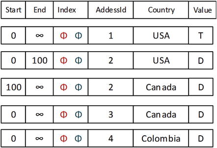
Figure 10-16. Sample table structure
By filtering on the two time frames, you can see one of the rows where AddressId = 2 falls out, leaving us with the two tables of the data.
The other very different part of the structure is how indexes work. The arrows in Figure 10-17 are index pointers. The part of the structure to find the first row is always a separate structure, but the physical record pointer just points to one row in the table. From there, all values that meet the criteria for a level in the index become a chain of rows.

Figure 10-17. Index pointers
In the example, one row from an index would point to the first row in the image, and the pointer would be followed for the second row. For the unique index, you instinctively might think there would never be a chain of rows, but this is not the case. For updates, you end up with multiple rows until the old rows are removed. Also, if using a hash index, it does not have uniqueness in the way it is implemented, it still needs to look for uniqueness. For any of the index types, the goal is generally to have no more than an average of 100 values in this chain to be scanned. If this is the case, it will be best to choose your index key columns so they are more unique (this should not be an issue with indexes you are using for a PRIMARY KEY/UNIQUE constraint.)
The index pointer structure is both limiting and empowering. It is limiting because you can only have the eight indexes. On the other hand, the leaf node of ALL indexes are the table’s data. So the primary benefit of a clustered index, that of not having to go fetch the rest of the data from a separate structure, is there for all in-memory OLTP indexes because of how they are structured. The downside is that we have a maximum of eight indexes per table.
Conceptually and structurally, things are very different, but for the most part, assuming you are designing and implementing memory-optimized tables, the most important thing is to understand the basic versioning structure to understand which index to choose when, and to really grok the differences in how concurrency is implemented.
Index Structure
When Microsoft created the in-memory OLTP engine, they didn’t just create one type of index like we had in the on-disk structures. There are two types (and you can use columnstore indexes as well). B-Tree based indexes are awesome structures, but they can be overkill when you simply need to do a single-row lookup. So Microsoft has given us (for in-memory objects only, so far) a new index type, a hash index.
In this section, we will look at the B-Tree based Bw-Tree indexes, as well as the new hash index types that are used for the in-memory OLTP structures.
Bw-Tree Indexes
The Bw-Tree index is, for all intents and purposes, very similar to the current B-Tree indexes that we have had in SQL Server since the very beginning. In the next two sections, I will look at the conceptual implementation and usage patterns for Bw-Tree indexes. In Figure 10-18, you can see the base structure of the index. There is a page mapping layer that contains the memory addresses of the pages of the index, and a B-Tree structure that conceptually is the same as on on-disk B-Tree, except the lower values of the tree are less than the key on the parent page. So, because Page 0 has C as the first entry, all values on the leftmost node will be C or less.

Figure 10-18. Bw-Tree index node pages
The values in the nodes of the index are not timestamped, and are maintained for all values. The values on the leaf nodes point to actual rows in the table. In our example table, this node set is an index that includes the Value column from the rows in our sample structure, as shown in Figure 10-19.
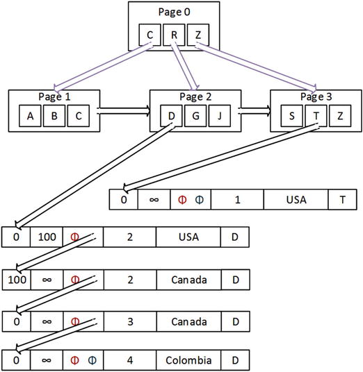
Figure 10-19. Bw-Tree index node pages linked to data
As shown in the intro section to memory-optimized tables, once you reach the value in the leaf node, it is the entry point into the internal linked list of index pointers. So all of the D values and versions we have are chained together row by row, and any older transactions are cleaned up as the engine can get to it.
Hash Indexes
Hashing is a well-tested concept in computer science, and has been used by the optimizer since SQL Server 7.0 to do joins on unindexed, unordered sets. The idea is that you create a function that takes (more or less) an infinite number of inputs, and outputs a finite, manageable “bucket” to match them in. For example, suppose you have the following data, and the ellipsis represents approximately 100 rows:
Name
-------------------
Amanda
Emma
Aria
Andrew
Addison
...
Jim
Linda
Max
Say all you ever need to do is find a name in the list. In a Bw-Tree, you would have the overhead of sorting the data, and perhaps also duplicating the data in the leaf pages of the index. In a hash index, you simply devise a function that will let you separate things into piles. As a human, you might use the first letter or letters of the name; or perhaps the length of the name, which gives you the following:
Name                HashBucket
------------------- --------------------
Amanda              6
Emma                4
Aria                4
Andrew              6
Addison             7
...
Jim                 3
Linda               5
Max                 3
You sort the data by the HashBucket, and then scan the bucket. This is very similar to what SQL Server will do with hash index structures, only with a hash function that will produce a lot greater variety in hash bucket values. In this section, I will look at conceptually how this is applied to hash indexes, and then cover some of the basics of creating and using hash indexes.
SQL Server basically implements hash buckets as one might do manually, using an unknown algorithm to do the hashing that you have no control over. (There is one hash algorithm for all data types.) You simply choose a number of buckets based on the expected number of unique values × approximately 2, which will be internally rounded up to the next highest power of 2. Then create the index and it does the work. Each bucket takes 8 bytes upon creation (or index rebuild), and does not change on its own. You have to resize the bucket count manually if your estimated number of unique values changes. Bear in mind that it is far better to have way too many hash buckets than too few. As stated in the intro section, if too many values are placed in the chain to scan, performance will degrade. The larger the number of hash buckets, the less likely this scenario will become.
As an example, in Figure 10-20, I have the structure that I started with earlier in this section, but now I have a hash index on the Country column. Note that two of the values hashed to the same value (how convenient for the example!). While you won’t see the internals, there are DMVs that will tell you the average bucket length, and it will almost never be 1, even when the index key is unique.
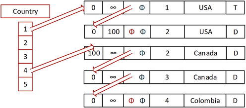
Figure 10-20. Sample hash index
In the data, USA hashes to bucket 1 (coincidentally, of course), and Canada and Colombia hash to 5. When SQL Server does a lookup in the index, it uses the same hash function that it used to put up the value, then it goes to the first row in the hash bucket, and scans all of the rows. So it would be three memory reads for Colombia, or Canada, or any other value that hashes to 4.
Indexing In-Memory OLTP Tables
Microsoft’s current prescription as of SQL Server 2016 for indexing in-memory OLTP tables is to start with the Bw-Tree based nonclustered indexes for pretty much all primary keys, unique keys, and all other indexes one might need. They are easier to create and have less maintenance, and they work well for most of the use cases one will have for in-memory OLTP tables.
It must be noted, however, that hash indexes will perform better as long as your use case is 100% single-value lookups like a primary key. This is largely due to fixed memory sizing and less processing needed to get to the head of the linked list of rows. But even then, how well the hashing function performs will depend on how many rows will end up needing scanned, as opposed to an NC Bw-Tree, where the scanned rows will be based strictly on all rows having the same index key value. Be certain that your bucket sizes are at least twice the number of unique values you have/expect and watch the chain length as previously mentioned. A very large number of values in a chain will start to degrade performance. Also remember that both indexes will have in their index chains data for expired rows that have not been cleaned up.
In the WideWorldImporters sample database, there are a few in-memory tables. We will use Warehouse.VehicleTemperatures in this section for a few plan demonstrations. It has the following structure:
CREATE TABLE Warehouse.VehicleTemperatures
(
        VehicleTemperatureID bigint IDENTITY(1,1) NOT NULL
                CONSTRAINT PK_Warehouse_VehicleTemperatures  PRIMARY KEY NONCLUSTERED,
        VehicleRegistration nvarchar(20) COLLATE Latin1_General_CI_AS NOT NULL,
        ChillerSensorNumber int NOT NULL,
        RecordedWhen datetime2(7) NOT NULL,
        Temperature decimal(10, 2) NOT NULL,
        FullSensorData nvarchar(1000) COLLATE Latin1_General_CI_AS NULL,
        IsCompressed bit NOT NULL,
        CompressedSensorData varbinary(max) NULL
) WITH ( MEMORY_OPTIMIZED = ON , DURABILITY = SCHEMA_AND_DATA );
It comes with 65,998 rows, and does not have any other indexes or foreign keys defined on the table itself other than the primary key.
The first thing you will notice is that not much is different in using these tables in simple queries (differences show up more in the next chapter with explicit transactions and concurrency, and even more when we get to Chapter 13 and I discuss a bit about native code versus interpreted T-SQL). Take the following query:
SELECT *
FROM   Warehouse.VehicleTemperatures;
The query plan is very much what you would expect:
|--Table Scan(OBJECT:([WideWorldImporters].[Warehouse].[VehicleTemperatures]))
Add in a primary key value:
SELECT *
FROM   Warehouse.VehicleTemperatures
WHERE  VehicleTemperatureID = 2332;
and you get an index seek and a parameterized plan:
|--Index Seek (OBJECT:([WideWorldImporters].[Warehouse].[VehicleTemperatures].
                                                       [PK_Warehouse_VehicleTemperatures]),
               SEEK:([WideWorldImporters].[Warehouse].[VehicleTemperatures].
               [VehicleTemperatureID]=CONVERT_IMPLICIT(bigint,[@1],0)) ORDERED FORWARD)
One difference you may see is a plan making more use of an index. For example, the query
SELECT *
FROM   Warehouse.VehicleTemperatures
WHERE  VehicleTemperatureID <> 0;
looks like a definite case for a full table scan. VehicleTemperature = 0 could only return 1 row, but the plan here is
|--Index Seek (OBJECT:([WideWorldImporters].[Warehouse].[VehicleTemperatures].
                                                       [PK_Warehouse_VehicleTemperatures]),
               SEEK:(
        [WideWorldImporters].[Warehouse].[VehicleTemperatures].[VehicleTemperatureID] < (0)
     OR [WideWorldImporters].[Warehouse].[VehicleTemperatures].[VehicleTemperatureID] > (0))
                                                                         ORDERED FORWARD)
In testing this query with or without an index, using STATISTIC TIME:
SELECT *
FROM   Warehouse.VehicleTemperatures WITH (INDEX = 0)
WHERE  VehicleTemperatureID <> 0;
the time difference was consistently slower using the index, but generally less than .1 second. The point of in-memory OLTP tables is to do small transactions, so they expect you to know what you are doing.
One of the reasons that the prescription is to use Bw-Tree indexes first is that hash indexes have only one purpose: single-row lookups. So if you need to do any sort of range query, hash indexes will not be helpful. For example, let’s add one to the RecordedWhen column:
ALTER TABLE  Warehouse.VehicleTemperatures
 ADD INDEX RecordedWhen                             --33000 distinct values,
    HASH (RecordedWhen) WITH (BUCKET_COUNT = 64000) --values are in powers of 2
Use an equality operator:
SELECT *
FROM   Warehouse.VehicleTemperatures
WHERE  RecordedWhen = ’2016-03-10 12:50:22.0000000’;
and the index is used:
|--Index Seek(
             OBJECT:([WideWorldImporters].[Warehouse].[VehicleTemperatures].[RecordedWhen]),
             SEEK:([WideWorldImporters].[Warehouse].[VehicleTemperatures].[RecordedWhen]
                                    =CONVERT_IMPLICIT(datetime2(7),[@1],0)) ORDERED FORWARD)
But even if the plan clearly can only return the same row, if it isn’t equality, it will use a scan and filter:
SELECT *
FROM   Warehouse.VehicleTemperatures
WHERE  RecordedWhen BETWEEN ’2016-03-10 12:50:22.0000000’ AND ’2016-03-10 12:50:22.0000000’;
This results in the following plan:
|--Filter(
           WHERE:([WideWorldImporters].[Warehouse].[VehicleTemperatures].[RecordedWhen]>=
                                                  CONVERT_IMPLICIT(datetime2(7),[@1],0)
                  AND
                  [WideWorldImporters].[Warehouse].[VehicleTemperatures].[RecordedWhen]<=
                                                  CONVERT_IMPLICIT(datetime2(7),[@2],0)))
       |--Table Scan(OBJECT:([WideWorldImporters].[Warehouse].[VehicleTemperatures]))
                                                                         ORDERED FORWARD)
If you have throughput needs that merit the use of the in-memory engine, you need to do testing to make sure that everything is working as you expect. In Chapter 11, we will see how even fast-looking queries can have a negative impact on concurrency when you don’t get your indexes right. In-memory OLTP is very new, and built for specific scenarios (hence “OLTP” in the title).
Columnstore Indexes
Columnstore indexes are, for the reporting specialist, an amazing tool. In this section I just want to give a very brief introduction to the structures so you can see conceptually the difference between columnstore indexes and typical row store indexes. A columnstore index is a form of columnar index. Columnar databases have been around for quite a while, which store all data by column. They have generally been great at implementing reporting solutions where you have to scan a lot of rows for every query, especially when dealing with lots of duplicate data. They are particularly useful when processing aggregates on large sets. The more columns in the object, and the fewer you need to use in the query, the greater the performance benefit. Figure 10-21 shows a conceptual diagram of the structure of a columnstore index.

Figure 10-21. Conceptual view of a columnstore index
The Column Segment blocks are ideally 1,048,576 rows each with each of the numbered sections representing a column, with each segment ordered by the rows in the table. They are different sized because each of the segments is compressed, much like you can compress normal data on a page, but instead of an 8K page, it is compressed over 1 million rows in a blob style storage.
Data in a columnstore index is not ordered, but is scanned for all usage in what is called “batch mode,” which processes data in ~900 at once, instead of the row-by-row mode used for typical row store indexes. In practice I have found in extreme cases (like a data warehouse fact table that has 120 columns and you are aggregating on 3) query performance can be orders of magnitude quicker.
The deltastore comes into play when you are modifying a table with a clustered columnstore index on it, new rows are dropped into the deltastore until you reach the 1,048,576-row threshold. The deltastore is basically a heap structure that will be scanned. Using the REBUILD or REORGANIZE commands of the ALTER INDEX command, you can manually push rows into the column segments also. I won’t dig too deep into the management of columnstore indexes in this book.
Updates to rows in a columnstore index are a delete from the columnstore index, and then the row is added to either the deltastore for a clustered columnstore, or to the last columnstore segment for a nonclustered version. So it will behoove you to avoid doing a lot of modifications if possible.
In SQL Server 2016, there are clustered and nonclustered columnstore indexes, and both are updateable, and both can be mixed with row store indexes. This improvement for 2016 enables some very advanced scenarios, which will be covered in Chapter 14. The most important benefit of mixing the indexes is that columnstore indexes are horrible at single-row lookups. This is because there is no uniqueness declared or enforced. This leads to every query being a scan of the structure.
Common OLTP Patterns of Index Usage
In this section I have gathered a few topics that are important to cover but did not fit the flow of the previous sections (sometimes because they needed multiple sections to be completed).
We will look at these topics:
- When to cluster on something other than the primary key: It may be the most common usage of the clustered index, but it isn’t always best.
- Indexing foreign keys: Foreign keys almost always represent a common path to retrieve data from a table, but do they always need indexed? Do they ever? (Yes they do, sometimes!)
- Indexed views: So far we have limited discussion to indexing tables, but you can index views in some cases to give you fast answers maintained by SQL Server’s code instead of yours.
- Compression: Fitting more data onto disk means less reads from disk, which is still the slowest part of a computer.
- Partitioning: Partitioning breaks up a table or index physically but still makes it look like one object to the end user. This allows for some coding and maintenance scenarios to be easier.
When to Cluster on Something Other Than the PRIMARY KEY
For an on-disk table, most every usage of a clustered index will be for the primary key, particularly when you are using a surrogate key. However, the clustered index won’t always be used for the surrogate key or even the primary key. Other possible uses can fall under the following types:
- Range queries: Having all the data in order usually makes sense when there’s data for which you often need to get a range, such as from A to F. An example where this can make sense is for the child rows in a parent–child relationship.
- Data that’s always accessed sequentially: Obviously, if the data needs to be accessed in a given order, having the data already sorted in that order will significantly improve performance.
- Queries that return large result sets: Since the data is stored with the clustered index, you can avoid the cost of the bookmark lookup, which often results in a table scan in any case.
- Child table foreign key references: In some cases, a table like InvoiceLineItem with basic structure (InvoiceLineItemId PK, InvoiceId FK, LineNumber, UNIQUE(InvoiceId, LineNumber)) may benefit greatly by clustering on the InvoiceId, even though it would not be unique. First you fetch the Invoice, then the InvoiceLineItem rows. Important to note is that sometimes you will end up using the surrogate key to fetch rows more than seems logical, so empirical testing and watching usage are important.
The choice of how to pick the clustered index depends on a couple of factors, such as how many other indexes will be derived from this index, how big the key for the index will be, and how often the value will change. When a clustered index value changes, every index on the table must also be touched and changed, and if the value can grow larger, well, then we might be talking page splits. This goes back to understanding the users of your data and testing the heck out of the system to verify that your index choices don’t hurt overall performance more than they help. Speeding up one query by using one clustering key could hurt all queries that use the nonclustered indexes, especially if you chose a large key for the clustered index.
Frankly, in an OLTP setting, in all but the most unusual cases, I start with a surrogate key for my clustering key, usually one of the integer types or sometimes even the unique identifier (GUID) type (ideally the sequential type), even if that is 16 bytes wide. I use the surrogate key because so many of the queries you do for modification (the general goal of the OLTP system) will typically access the data via the primary key. You then just have to optimize retrievals, which should also be of generally small numbers of rows, and doing so is usually pretty easy.
To reiterate an important point, it is also very good to use the clustered index on a value like a monotonically increasing surrogate so that page splits over the entire index are greatly decreased on inserts. The table grows only on one end of the index, and while it does need to be rebuilt occasionally using ALTER INDEX REORGANIZE or ALTER INDEX REBUILD, you don’t end up with page splits all over the table. You can decide which to do by using the criteria stated by SQL Server Books Online. By looking in the dynamic management view sys.dm_db_index_physical_stats, you can use REBUILD on indexes with greater than 30% fragmentation and use REORGANIZE. We will discuss this more in the “Indexing Dynamic Management View Queries” section later in the chapter.
Indexing Foreign Keys
Foreign key columns are a special case where we often need an index of some type. This is true both in on-disk and in-memory tables. We build foreign keys so we can match up rows in one table to rows in another. For this, we have to take a value in one table and match it to another.
In an OLTP database that has proper constraints on alternate keys, often, we won’t may not need to index foreign keys beyond what we’re given with the unique indexes that are built as part of the structure of the database. This is probably why SQL Server doesn’t implement indexes for us when creating a foreign key constraint.
However, it’s important to make sure that any time you have a foreign key constraint declared, there’s the potential for need of an index. Often when you have a parent table with specific values, you may want to see the children of the row. A special and important case where this type of access is essential is when you have to delete the parent row in any relationship, even one of a domain type that has a very low cardinality. If in doubt, it is not a terrible practice to add indexes to foreign keys by default, and during testing use one of the queries in the upcoming “Indexing Dynamic Management View Queries” section to identify how or if indexes are being used.
Say you have five values in the parent table and 500 million in the child. For example, consider the case of a click log for a sales database, a snippet of which is shown in Figure 10-22.

Figure 10-22. Sample foreign key relationship
Consider that you want to delete a clickType row that someone added inadvertently. Creating the row took several milliseconds. Deleting it shouldn’t take long at all, right? Well, even if there isn’t a matching value in the table, if you don’t have an index on the foreign key in the siteClickLog table, it may take just over 10 seconds longer than eternity. Even though the value doesn’t exist in the table, the query processor would need to touch and check all 500 million rows for the value. From the statistics on the column, the query processor can guess how many rows might exist, but it can’t definitively know that there is or is not a value because statistics are maintained asynchronously. (Ironically, because it is an existence search, the query processor could fail quickly on the first row it checked, but to successfully delete the row, every child row must be touched.)
However, if you have an index, deleting the row (or knowing that you can’t delete it) will take a very short period of time, because in the upper pages of the index, you’ll have all the unique values in the index, in this case, five values. There will be a fairly substantial set of leaf pages for the index, but only one page in each index level, usually no more than three or four pages, will need to be touched before the query processor can determine the existence of a row out of millions of rows. When NO ACTION is specified for the relationship, if just one row is found, the operation could be stopped. If you have cascading operations enabled for the relationship, the cascading options will need the index to find the rows to cascade to.
This adds more decisions when building indexes. Is the cost of building and maintaining the index during creation of millions of siteClickLog rows justified, or do you just bite the bullet and do deletes during off-hours? Add a trigger such as the following, ignoring error handling in this example for brevity:
CREATE TRIGGER clickType$insteadOfDelete
ON clickType
INSTEAD OF DELETE
AS
    INSERT INTO clickType_deleteQueue (clickTypeId)
    SELECT clickTypeId
    FROM   deleted;
Then, let your queries that return lists of clickType rows check this table when presenting rows to the users:
SELECT code, description, clickTypeId
FROM   clickType
WHERE  NOT EXISTS (SELECT *
                   FROM   clickType_deleteQueue
                   WHERE  clickType.clickTypeId =
                              clickType_deleteQueue.clickTypeId);
Now, assuming all code follows this pattern, the users will never see the value, so it won’t be an issue (at least not in terms of values being used; performance will suffer obviously). Then, you can delete the row in the wee hours of the morning without building the index. Whether or not an index proves useful generally depends on the purpose of the foreign key. I’ll mention specific types of foreign keys individually, each with their own signature usage:
- Domain tables: Used to implement a defined set of values and their descriptions
- Ownership relationships: Used to implement a multivalued attribute of the parent
- Many-to-many resolution table relationships: Used to implement a many-to-many relationship physically
- One-to-one relationships: Cases where a parent may have only a single value in the related table
We’ll look at examples of these types and discuss when it’s appropriate to index them before the typical trial-and-error performance tuning, where the rule of thumb is to add indexes to make queries faster, while not slowing down other operations that create data.
In all cases, deleting the parent row requires a table scan of the child if there’s no index on the child row. This is an important consideration if there are deletes.
You use a domain table to enforce a domain using a table, rather than using a scalar value with a constraint. This is often done to enable a greater level of data about the domain value, such as a descriptive value. For example, consider the tables in Figure 10-23.

Figure 10-23. Sample domain table relationship
In this case, there are a small number of rows in the productType table. It’s unlikely that an index on the product.productTypeCode column would be of any value in a join, because you’ll generally be getting a productType row for every row you fetch from the product table.
What about the other direction, when you want to find all products of a single type? This can be useful if there aren’t many products, but in general, domain type tables don’t have enough unique values to merit an index. The general advice is that tables of this sort don’t need an index on the foreign key values, by default. Of course, deleting productType rows would need to scan the entire productType.
On the other hand, as discussed earlier in the chapter, sometimes an index can be useful when there are limited numbers of some value. For example, consider a user to userStatus relationship illustrated in Figure 10-24.

Figure 10-24. Sample domain table relationship with low cardinality
In this case, most users would be in the database with an active status. However, when a user is deactivated, you might need to do some action for that user. Since the number of inactive users would be far fewer than active users, it might be useful to have an index (possibly a filtered index) on the UserStatusCode column for that purpose.
Some tables have no meaning without the existence of another table and pretty much exist to as part of another table (due to the way relational design works). When I am thinking about an ownership relationship, I am thinking of relationships that implement multivalued attributes for a row, just like an array in a procedural language does for an object. The main performance characteristic of this situation is that most of the time when the parent row is retrieved, the child rows are retrieved as well. You’ll be less likely to need to retrieve a child row and then look for the parent row.
For example, take the case of an invoice and its line items in Figure 10-25.

Figure 10-25. Sample ownership relationship
In this case, it’s essential to have an index on the invoiceLineItem.invoiceId column, probably as part of a UNIQUE constraint. A large amount of access to the invoiceLineItem table results from a user’s need to get an invoice first. This situation is also ideal for an index because, usually, it will turn out to be a very selective index (unless you have large numbers of items and few sales).
Note that you should already have a UNIQUE constraint (and a unique index as a consequence of this) on the alternate key for the table—in this case, invoiceId and invoiceLineNumber. Therefore, you probably wouldn’t need to have an index on just invoiceId. What might be in question would be whether or not the index on invoiceId and invoiceLineNumber ought to be clustered, as I noted in the previous section about when to cluster on a non-surrogate value. If you do most of your SELECT operations using the invoiceId, this actually can be a good idea. However, you should be careful in this case because you can actually do a lot more fetches on the primary key value, since UPDATE and DELETE operations start out performing like a SELECT before the modification. For example, the application may end up doing one query to get the invoice line items and then update each row individually to do some operation. So always watch the activity in your database and tune accordingly.
Many-to-Many Resolution Table Relationships
When we have a many-to-many relationship, there certainly needs to be an index on the two migrated keys from the two parent tables. Using an example that we used in Chapter 7, with a many-to-many relationship between tables that hold games a person owns, the relationship between gamePlatform and game is shown in Figure 10-26.

Figure 10-26. Sample many-to-many relationship
In this case, you should already have a unique index on gamePlatformId and gameId, and one of the two will necessarily be first in the composite index. If you need to search for both keys independently of one another, you may want to create an index on each column individually (or at least the column that is listed second in the uniqueness constraint’s index).
Take this example. If we usually look up a game by name (which would be alternate key indexed) and then get the platforms for this game, an index only on gameInstance.gameId would be much more useful and two-thirds the size of the alternate key index (assuming a clustering key of gameInstanceId).
One-to-one relationships generally require some form of unique index on the key in the parent table as well as on the migrated key in the child table. For example, consider the subclass example of a bankAccount, shown in Figure 10-27.

Figure 10-27. Sample one-to-one relationship
In this case, because these are one-to-one relationships, and there are already indexes on the primary key of each table, no other indexes would need to be added to effectively implement the relationship.
Indexed Views
I mentioned the use of persisted calculated columns in Chapter 6 for optimizing denormalizations for a single row, but sometimes, your denormalizations need to span multiple rows and include things like summarizations. In this section, I will introduce a way to take denormalization to the next level, using indexed views.
Indexing a view basically takes the virtual structure of the view and makes it a physical entity, albeit one managed completely by the query processor. The data to resolve queries with the view is generated as data is modified in the table, so access to the results from the view is just as fast as if it were an actual table. Indexed views give you the ability to build summary tables without any kind of manual operation or trigger; SQL Server automatically maintains the summary data for you. Creating indexed views is (more or less) as easy as writing a query.
The benefits are twofold when using indexed views. First, when you use an indexed view directly in any edition of SQL Server, it does not have to do any calculations (editions less than Enterprise must specify NOEXPAND as a hint). Second, in Enterprise edition or greater (plus Developer edition), SQL Server automatically considers the use of an indexed view whenever you execute any query, even if the query doesn’t reference the view but the code you execute uses the same aggregates. SQL Server accomplishes this index view assumption by matching the executed query to each indexed view to see whether that view already has the answer to something you are asking for.
For example, we could create the following view on the product and sales tables in the WideWorldImporters database. Note that only schema-bound views can be indexed as this makes certain that the tables and structures that the index is created upon won’t change underneath the view. (A more complete list of requirements is presented after the example.)
CREATE VIEW Warehouse.StockItemSalesTotals
WITH SCHEMABINDING
AS
SELECT StockItems.StockItemName,
                                 --ISNULL because expression can’t be nullable
       SUM(OrderLines.Quantity * ISNULL(OrderLines.UnitPrice,0)) AS TotalSalesAmount,
       COUNT_BIG(*) AS TotalSalesCount--must use COUNT_BIG for indexed view
FROM  Warehouse.StockItems
          JOIN Sales.OrderLines
                 ON  OrderLines.StockItemID = StockItems.StockItemID
GROUP  BY StockItems.StockItemName;
This would do the calculations at execution time. We run the following query:
SELECT *
FROM   Warehouse.StockItemSalesTotals;
The plan looks like…well, like five operators that go on for a while and would be really hard to read in text. An image is provided in Figure 10-28. It loses a lot of fidelity from the textual plans, but it might save a tree.

Figure 10-28. Query plan image from using the view
This is a big plan for such a small query, for sure, and it’s hard to follow. It scans the OrderLines table, computes our scalar values, and then does a hash match aggregate and a hash match join to join the two sets together. For further reading on the join types, again consider a book in Kalen Delaney’s SQL Server Internals series.
This only returns 227 rows in this sample database, but say this query wasn’t fast enough, or it used too many resources to execute, or it was used extremely often. In this case, we might add an index on the view. Note that it is a clustered index, as the data pages will be ordered based on the key we chose. Consider your structure of the index just like you would on a physical table.
CREATE UNIQUE CLUSTERED INDEX XPKStockItemSalesTotals on
                      Warehouse.StockItemSalesTotals(StockItemName);
SQL Server would then materialize the view and store it. Now, our queries to the view will be very fast. However, although we’ve avoided all the coding issues involved with storing summary data, we have to keep our data up to date. Every time data changes in the underlying tables, the index on the view changes its data, so there’s a performance hit in maintaining the index for the view. Hence, indexing views means that performance is great for reading but not necessarily for updating.
Now, run the query again and the plan looks like the following:
|--Clustered Index Scan
              (OBJECT:([WideWorldImporters].[Warehouse].[StockItemSalesTotals].
                                                              [XPKStockItemSalesTotals]))
No big deal, right? We expected this result because we directly queried the view. On my test system, running Developer edition (which is functionally comparable to Enterprise edition), you get a great insight into how cool this feature is by running the following query, which is basically our original query with a division operator between the two factors:
SELECT StockItems.StockItemName,
       SUM(OrderLines.Quantity * ISNULL(OrderLines.UnitPrice,0)) / COUNT_BIG(*)
                                                               AS AverageSaleAmount
FROM  Warehouse.StockItems
          JOIN Sales.OrderLines
                 ON  OrderLines.StockItemID = StockItems.StockItemID
GROUP  BY StockItems.StockItemName;
We’d expect the plan for this query to be the same as the first query of the view was, because we haven’t referenced anything other than the base tables, right? I already told you the answer, so here’s the plan:
|--Compute Scalar
    (DEFINE:([Expr1006]=
               [WideWorldImporters].[Warehouse].[StockItemSalesTotals].[TotalSalesAmount]
    /CONVERT_IMPLICIT(decimal(19,0),[WideWorldImporters].[Warehouse].[StockItemSalesTotals].
                                                                      [TotalSalesCount],0)))
       |--Clustered Index Scan
              (OBJECT:([WideWorldImporters].[Warehouse].[StockItemSalesTotals].
                                                                 [XPKStockItemSalesTotals]))
There is a scalar compute that does our math, but instead you will notice that the plan references the StockItemSalesTotals indexed view, and we did not reference it directly in our query. The ability to use the optimizations from an indexed view indirectly is a neat feature that allows you to build in some guesses as to what ad hoc users will be doing with the data and give them performance they didn’t even ask for.
![]() Tip The indexed view feature in Enterprise edition and greater can also come in handy for tuning third-party systems that work on an API that is not tunable in a direct manner (that is, to change the text of a query to make it more efficient).
Tip The indexed view feature in Enterprise edition and greater can also come in handy for tuning third-party systems that work on an API that is not tunable in a direct manner (that is, to change the text of a query to make it more efficient).
There are some pretty heavy caveats, though. The restrictions on what can be used in a view, prior to it being indexed, are fairly tight. The most important things that cannot be done are as follows:
- Use the SELECT * syntax—columns must be explicitly named.
- Use a CLR user-defined aggregate.
- Use UNION, EXCEPT, or INTERSECT in the view.
- Use any subqueries.
- Use any outer joins or recursively join back to the same table.
- Specify TOP in the SELECT clause.
- Use DISTINCT.
- Include a SUM() function if it references more than one column.
- Use COUNT(*), though COUNT_BIG(*) is allowed.
- Use almost any aggregate function against a nullable expression.
- Reference any other views, or use CTEs or derived tables.
- Reference any nondeterministic functions.
- Reference data outside the database.
- Reference tables owned by a different owner.
And this isn’t all. You must meet several pages of requirements, documented in SQL Server Books Online in the section “Create Indexed Views” (msdn.microsoft.com/en-us/library/ms191432.aspx). However, these are the most significant ones that you need to consider before using indexed views.
Although this might all seem pretty restrictive, there are good reasons for all these rules. Maintaining the indexed view is analogous to writing our own denormalized data maintenance functions. Simply put, the more complex the query to build the denormalized data, the greater the complexity in maintaining it. Adding one row to the base table might cause the view to need to recalculate, touching thousands of rows.
Indexed views are particularly useful when you have a view that’s costly to run but the data on which it’s based doesn’t change a tremendous amount. As an example, consider a decision-support system where you load data once a day. There’s overhead either maintaining the index or, possibly, just rebuilding it, but if you can build the index during off-hours, you can omit the cost of redoing joins and calculations for every view usage.
![]() Tip With all the caveats, indexed views can prove useless for some circumstances. An alternative method is to materialize the results of the data by inserting the data into a permanent table, in any case where you can handle some latency on the data
Tip With all the caveats, indexed views can prove useless for some circumstances. An alternative method is to materialize the results of the data by inserting the data into a permanent table, in any case where you can handle some latency on the data
Compression
I mentioned compression when we looked at columnstore indexes. In a normal index (which includes clustered, heaps, and B-Trees), SQL Server can save space by storing all of your data like it was a variable-sized type, yet in usage, the data will appear and behave like a fixed length type. In Appendix A, I will note how compression will affect each datatype individually, or if you want to see a list that may show any recent changes, you can check SQL Server Books Online for the topic of “Row Compression Implementation” (msdn.microsoft.com/en-us/library/cc280576.aspx).
For example, if you stored the value of 100 in an int column, SQL Server needn’t use all 4 bytes; it can store the value 100 in the same amount of space as a tinyint. So instead of taking a full 4 bytes, SQL Server can simply use 8 bits (1 byte). Another case is when you use a fixed length type like a char(30) column but store only two characters; 28 characters could be saved, and the data padded as it is used.
This datatype-level compression is part of row compression, where each row in the table will be compressed as datatypes allow, shrinking the size on disk, but not making any major changes to the page structure. Row compression is a very interesting option for many databases that use lots of fixed length data (for example, integers, especially for surrogate keys).
SQL Server also includes an additional compression capability called page compression. With page compression, first the data is compressed in the same manner as row compression, and then, the storage engine does a couple of interesting things to compress the data on a page:
- Prefix compression: The storage engine looks for repeated values in a value (like ’0000001’ and compresses the prefix to something like 6-0 (six zeros).
- Dictionary compression: For all values on the page, the storage engine looks for duplication, stores the duplicated value once, and then stores pointers on the data pages where the duplicated values originally resided.
You can apply data compression to your tables and indexes with the CREATE TABLE, ALTER TABLE, CREATE INDEX, and ALTER INDEX syntaxes. As an example, I will create a simple table, called test, and enable page compression on the table, row compression on a clustered index, and page compression on another index.
USE Tempdb
GO
CREATE TABLE dbo.TestCompression
(
    TestCompressionId int,
    Value  int
)
WITH (DATA_COMPRESSION = ROW) -- PAGE or NONE
    ALTER TABLE testCompression REBUILD WITH (DATA_COMPRESSION = PAGE);
CREATE CLUSTERED INDEX Value
   ON testCompression (Value) WITH ( DATA_COMPRESSION = ROW );
ALTER INDEX Value  ON testCompression REBUILD WITH ( DATA_COMPRESSION = PAGE );
![]() Note The syntaxes of the CREATE INDEX and CREATE TABLE commands allow for compression of the partitions of an index in different manners. I mention partitioning in the next section of the chapter. For full syntax, refer to SQL Server Books Online.
Note The syntaxes of the CREATE INDEX and CREATE TABLE commands allow for compression of the partitions of an index in different manners. I mention partitioning in the next section of the chapter. For full syntax, refer to SQL Server Books Online.
Giving advice on whether to use compression is not really possible without knowing the factors that surround your actual situation. One tool you should use is the system procedure—sp_estimate_data_compression_savings—to check existing data to see just how compressed the data in the table or index would be after applying compression, but it won’t tell you how the compression will positively or negatively affect your performance. There are trade-offs to any sorts of compression. CPU utilization will go up in most cases, because instead of directly using the data right from the page, the query processor will have to translate the values from the compressed format into the uncompressed format that SQL Server will use. On the other hand, if you have a lot of data that would benefit from compression, you could possibly lower your I/O enough to make doing so worth the cost. Frankly, with CPU power growing by leaps and bounds with multiple-core scenarios these days and I/O still the most difficult to tune, compression could definitely be a great thing for many systems. However, I suggest testing with and without compression before applying it in your production systems.
Partitioning
Partitioning allows you to break an index/table into multiple physical structures that look to the end user to be only one by breaking them into more manageable chunks. Partitioning can allow SQL Server to scan data from different processes, enhancing opportunities for parallelism.
Partitioning allows you to define physical divisions within your table structure. Instead of making a physical table for each partition, you define, at the DDL level, the different partitions of the table. Internally, the table is broken into the partitions based on a scheme that you set up.
At query time, SQL Server can then dynamically scan only the partitions that need to be searched, based on the criteria in the WHERE clause of the query being executed. I am not going to describe partitioning too much, but I felt that it needed a mention in this edition of this book as a tool at your disposal with which to tune your databases, particularly if they are very large or very active. In-memory tables can participate in a partitioning scheme, and not every partition needs to be in-memory to do so. For deeper coverage, I would suggest you consider one of Kalen Delaney’s SQL Server Internals books. They are the gold standard in understanding the internals of SQL Server.
I will, however, present the following basic example of partitioning. Use whatever database you desire. The example is that of a sales order table. I will partition the sales into three regions based on the order date. One region is for sales before 2006, another for sales between 2006 and 2007, and the last for 2007 and later. The first step is to create a partitioning function. You must base the function on a list of values, where the VALUES clause sets up partitions that the rows will fall into based on the smalldatetime values that are presented to it, for our example:
USE Tempdb;
GO
--Note that the PARTITION FUNCTION is not a schema owned object
CREATE PARTITION FUNCTION PartitionFunction$Dates (date)
AS RANGE LEFT FOR VALUES (’20140101’,’20150101’);
                  --set based on recent version of
                  --WideWorldImporters.Sales.Orders table to show
                  --partition utilization
Specifying the function as RANGE LEFT says that the values in the comma-delimited list should be considered the boundary on the side listed. So in this case, the ranges would be as follows:
- value <= ’20131231’
- value >= ’20140101’ and value <= ’20141231’
- value >= ’20150101’
Next, use that partition function to create a partitioning scheme:
CREATE PARTITION SCHEME PartitonScheme$dates
                AS PARTITION PartitionFunction$dates ALL to ( [PRIMARY] );
This will let you know
Partition scheme ’PartitonScheme$dates’ has been created successfully. ’PRIMARY’ is marked as the next used filegroup in partition scheme ’PartitonScheme$dates’.
With the CREATE PARTITION SCHEME command, you can place each of the partitions you previously defined on a specific filegroup. I placed them all on the same filegroup for clarity and ease, but in practice, you may want them on different filegroups, depending on the purpose of the partitioning. For example, if you were partitioning just to keep the often-active data in a smaller structure, placing all partitions on the same filegroup might be fine. But if you want to improve parallelism or be able to just back up one partition with a filegroup backup, you would want to place your partitions on different filegroups.
Next, you can apply the partitioning to a new table. You’ll need a clustered index involving the partition key. You apply the partitioning to that index. Following is the statement to create the partitioned table:
CREATE TABLE dbo.Orders
(
    OrderId     int,
    CustomerId  int,
    OrderDate  date,
    CONSTRAINT PKOrder PRIMARY KEY NONCLUSTERED (OrderId) ON [Primary],
    CONSTRAINT AKOrder UNIQUE CLUSTERED (OrderId, OrderDate)
) ON PartitonScheme$dates (OrderDate);
Next, load some data from the WideWorldImporters.Sales.Orders table to make looking at the metadata more interesting. You can do that using an INSERT statement such as the following:
INSERT INTO dbo.Orders (OrderId, CustomerId, OrderDate)
SELECT OrderId, CustomerId, OrderDate
FROM  WideWorldImporters.Sales.Orders;
You can see what partition each row falls in using the $partition function. You suffix the $partition function with the partition function name and the name of the partition key (or a partition value) to see what partition a row’s values are in, for example:
SELECT *, $partition.PartitionFunction$dates(orderDate) as partition
FROM   dbo.Orders;
You can also view the partitions that are set up through the sys.partitions catalog view. The following query displays the partitions for our newly created table:
SELECT  partitions.partition_number, partitions.index_id,
        partitions.rows, indexes.name, indexes.type_desc
FROM    sys.partitions as partitions
           JOIN sys.indexes as indexes
               on indexes.object_id = partitions.object_id
                   and indexes.index_id = partitions.index_id
WHERE   partitions.object_id = object_id(’dbo.Orders’);
This will return the following:
partition_number index_id    rows        name           type_desc
---------------- ----------- ----------- -------------- ---------------------
1                1           19547       AKSalesOrder   CLUSTERED
2                1           21198       AKSalesOrder   CLUSTERED
3                1           32850       AKSalesOrder   CLUSTERED
1                2           73595       PKSalesOrder   NONCLUSTERED
Partitioning is not a general-purpose tool that should be used on every table. However, partitioning can solve a good number of problems for you, if need be:
- Performance: If you only ever need the past month of data out of a table with three years’ worth of data, you can create partitions of the data where the current data is on a partition and the previous data is on a different partition.
- Rolling windows: You can remove data from the table by dropping a partition, so as time passes, you add partitions for new data and remove partitions for older data (or move to a different archive table). Multiple uniqueness constraints can be difficult using rolling windows, so be sure to cover all of your uniqueness needs in some manner.
- Maintenance: Some maintenance can be done at the partition level rather than for the entire table, so once partition data is read-only, you may not need to maintain any longer. Some caveats do apply that are subject to change, so I will leave it to you to check the documentation.
Indexing Dynamic Management View Queries
In this section, I want to provide a couple of queries that use the dynamic management views that you may find handy when you are tuning your system or index usage. In SQL Server 2005, Microsoft added a set of objects (views and table-valued functions) to SQL Server that gave us access to some of the deep metadata about the performance of the system. A great many of these objects are useful for managing and tuning SQL Server, and I would suggest you do some reading about these objects (not to be overly self-serving, but the book Performance Tuning with SQL Server Dynamic Management Views (High Performance SQL Server) by Tim Ford and myself, published by Simple-Talk in 2010, is my favorite book on the subject, even though it is kind of old at this point). I do want to provide you with some queries that will likely be quite useful for you when doing any tuning using indexes.
The first query we’ll discuss provides a peek at what indexes the optimizer thought might be useful for queries (on-disk and in-memory). It can be very helpful when tuning a database, particularly a very busy database executing thousands of queries a minute. I have personally used this query to tune third-party systems where I didn’t have a lot of access to the queries in the system and using Extended Events was simply far too cumbersome with too many queries to effectively tune manually.
This query uses three of the dynamic management views that are part of the missing index family of objects:
- sys.dm_db_missing_index_groups: This relates missing index groups with the indexes in the group.
- sys.dm_db_missing_index_group_stats: This provides statistics of how much the indexes in the group would have helped (and hurt) the system.
- sys.dm_db_missing_index_details: This provides information about the index that the optimizer would have chosen to have available.
The query is as follows. I won’t attempt to build a scenario where you can test this functionality in this book, but run the query on one of your development servers and check the results. The results will likely make you want to run it on your production server.
SELECT ddmid.statement AS object_name, ddmid.equality_columns, ddmid.inequality_columns,
       ddmid.included_columns,  ddmigs.user_seeks, ddmigs.user_scans,
       ddmigs.last_user_seek, ddmigs.last_user_scan, ddmigs.avg_total_user_cost,
       ddmigs.avg_user_impact, ddmigs.unique_compiles
FROM   sys.dm_db_missing_index_groups AS ddmig
         JOIN sys.dm_db_missing_index_group_stats AS ddmigs
                ON ddmig.index_group_handle = ddmigs.group_handle
         JOIN sys.dm_db_missing_index_details AS ddmid
                ON ddmid.index_handle = ddmig.index_handle
ORDER BY ((user_seeks + user_scans) * avg_total_user_cost * (avg_user_impact * 0.01)) DESC;
The query returns the following information about the structure of the index that might have been useful:
- object_name: This is the database and schema qualified object name of the object that the index would have been useful on. The data returned is for all databases on the entire server
- equality_columns: These are the columns that would have been useful, based on an equality predicate. The columns are returned in a comma-delimited list.
- inequality_columns: These are the columns that would have been useful, based on an inequality predicate (which as we have discussed is any comparison other than column = value or column in (value, value1)).
- included_columns: These columns, if added to the index via an INCLUDE clause, would have been useful to cover the query results and avoid a key lookup operation in the plan. Ignore these for in-memory queries as all columns are essentially included due to the structure of these tables.
As discussed earlier, the equality columns would generally go first in the index column definition, but it isn’t guaranteed that that will make the correct index. These are just guidelines, and using the next DMV query I will present, you can discover if the index you create turns out to be of any value.
- unique_compiles: The number of plans that have been compiled that might have used the index
- user_seeks: The number of seek operations in user queries that might have used the index
- user_scans: The number of scan operations in user queries that might have used the index
- last_user_seek: The last time that a seek operation might have used the index
- last_user_scan: The last time that a scan operation might have used the index
- avg_total_user_cost: Average cost of queries that could have been helped by the group of indexes
- avg_user_impact: The percentage of change in cost that the index is estimated to make for user queries
Note that I sorted the query results as (user_seeks + user_scans) * avg_total_user_cost * (avg_user_impact * 0.01) based on the initial blog article I read about using the missing indexes, “Fun for the Day – Automated Auto-Indexing” (blogs.msdn.microsoft.com/queryoptteam/2006/06/01/fun-for-the-day-automated-auto-indexing/). I generally use some variant of that to determine what is most important. For example, I might use order by (user_seeks + user_scans) to see what would have been useful the most times. It really just depends on what I am trying to scan; with all such queries, it pays to try out the query and see what works for your situation.
To use the output, you can create a CREATE INDEX statement from the values in the four structural columns. Say you received the following results:
object_name                          equality_columns               inequality_columns
------------------------------------ ------------------------------ --------------------
databasename.schemaname.tablename    columnfirst, columnsecond      columnthird
included_columns
-------------------------
columnfourth, columnfifith
You could build the following index to satisfy the need:
CREATE INDEX XName ON databaseName.schemaName.TableName(columnfirst, columnsecond, columnthird) INCLUDE (columnfourth, columnfifith);
Next, see if it helps out performance in the way you believed it might. And even if you aren’t sure of how the index might be useful, create it and just see if it has an impact.
Books Online lists the following limitations to consider:
- It is not intended to fine-tune an indexing configuration.
- It cannot gather statistics for more than 500 missing index groups.
- It does not specify an order for columns to be used in an index.
- For queries involving only inequality predicates, it returns less accurate cost information.
- It reports only include columns for some queries, so index key columns must be manually selected.
- It returns only raw information about columns on which indexes might be missing. This means the information returned may not be sufficient by itself without additional processing before building the index.
- It does not suggest filtered indexes.
- It can return different costs for the same missing index group that appears multiple times in XML showplans.
- It does not consider trivial query plans.
Probably the biggest concern is that it can specify a lot of overlapping indexes, particularly when it comes to included columns, since each entry could have been specifically created for distinct queries. For very busy systems, you may find a lot of the suggestions include very large sets of include columns that you may not want to implement.
However, limitations aside, the missing index dynamic management views are amazingly useful to help you see places where the optimizer would have liked to have an index and one didn’t exist. This can greatly help diagnose very complex performance/indexing concerns, particularly ones that need a large amount of INCLUDE columns to cover complex queries. This feature is turned on by default and can only be disabled by starting SQL Server with a command-line parameter of –x. This will, however, disable keeping several other statistics like CPU time and cache-hit ratio stats.
Using this feature and the query in the next section that can tell you what indexes have been used, you can use these index suggestions in an experimental fashion, just building a few of the indexes and see if they are used and what impact they have on your performance-tuning efforts.
On-Disk Index Utilization Statistics
The second query gives statistics on how an index has been used to resolve queries. Most importantly, it tells you the number of times a query was used to find a single row (user_seeks), a range of values, or to resolve a non-unique query (user_scans), if it has been used to resolve a bookmark lookup (user_lookups), and how many changes to the index (user_updates). If you want deeper information on how the index was modified, check sys.dm_db_index_operational_stats. The query makes use of the sys.dm_db_index_usage_stats object that provides just what the names says, usage statistics:
SELECT OBJECT_SCHEMA_NAME(indexes.object_id) + ’.’ +
       OBJECT_NAME(indexes.object_id) as objectName,
       indexes.name,
       case when is_unique = 1 then ’UNIQUE ’
              else ’’ end + indexes.type_desc as index_type,
       ddius.user_seeks, ddius.user_scans, ddius.user_lookups,
       ddius.user_updates, last_user_lookup, last_user_scan, last_user_seek,last_user_update
FROM   sys.indexes
          LEFT OUTER JOIN sys.dm_db_index_usage_stats ddius
               ON indexes.object_id = ddius.object_id
                   AND indexes.index_id = ddius.index_id
                   AND ddius.database_id = DB_ID()
ORDER  BY ddius.user_seeks + ddius.user_scans + ddius.user_lookups DESC;
The query (as written) is database dependent in order to look up the name of the index in sys.indexes, which is a database-level catalog view. The sys.dm_db_index_usage_stats object returns all indexes (including heaps and the clustered index) from the entire server (there will not be a row for sys.dm_db_index_usage_stats unless the index has been used since the last time the server has been started). The query will return all indexes for the current database (since the DMV is filtered on DB_ID() in the join criteria) and will return
- object_name: Schema-qualified name of the table.
- index_name: The name of the index (or table) from sys.indexes.
- index_type: The type of index, including uniqueness and clustered/nonclustered.
- user_seeks: The number of times the index has been used in a user query in a seek operation (one specific row).
- user_scans: The number of times the index has been used by scanning the leaf pages of the index for data.
- user_lookups: For clustered indexes only, this is the number of times the index has been used in a bookmark lookup to fetch the full row. This is because nonclustered indexes use the clustered indexes key as the pointer to the base row.
- user_updates: The number of times the index has been modified due to a change in the table’s data.
- last_user_seek: The date and time of the last user seek operation.
- last_user_scan: The date and time of the last user scan operation.
- last_user_lookup: The date and time of the last user lookup operation.
- last_user_update: The date and time of the last user update operation.
There are also columns for system utilizations of the index in operations such as automatic statistics operations: system_seeks, system_scans, system_lookups, system_updates, last_system_seek, last_system_scan, last_system_lookup, and last_system_update.
This is one of the most interesting views that I often use in performance tuning. It gives you the ability to tell when indexes are not being used. It is easy to see when an index is being used by a query by simply looking at the plan. But now, using this dynamic management view, you can see over time what indexes are used, not used, and, probably more importantly, updated many, many times without ever being used.
One of the biggest tasks for the DBA of a system is to make sure that the structures of indexes and tables are within a reasonable tolerance. You can decide whether to reorganize or to rebuild using the criteria stated by SQL Server Books Online in the topic for the dynamic management view sys.dm_db_index_physical_stats. You can check the FragPercent column and REBUILD indexes with greater than 30% fragmentation and REORGANIZE those that are just lightly fragmented.
SELECT  s.[name] AS SchemaName,
        o.[name] AS TableName,
        i.[name] AS IndexName,
        f.[avg_fragmentation_in_percent] AS FragPercent,
        f.fragment_count ,
        f.forwarded_record_count --heap only
FROM sys.dm_db_index_physical_stats(DB_ID(), NULL, NULL, NULL, DEFAULT) f
        JOIN sys.indexes i
             ON f.[object_id] = i.[object_id] AND f.[index_id] = i.[index_id]
        JOIN sys.objects o
             ON i.[object_id] = o.[object_id]
        JOIN sys.schemas s
             ON o.[schema_id] = s.[schema_id]
WHERE o.[is_ms_shipped] = 0
  AND i.[is_disabled] = 0; -- skip disabled indexes
sys.dm_db_index_physical_stats will give you a lot more information about the internal physical structures of your tables and indexes than I am making use of here. If you find you are having a lot of fragmentation, adjusting the fill factor of your tables or indexes (specified as a percentage of page size to leave empty for new rows) in CREATE INDEX and PRIMARY KEY and UNIQUE constraint CREATE/ALTER DDL statements can help tremendously. How much space to leave will largely depend on your exact situation, but minimally, you want to leave approximately enough space for one full additional row to be added to each page.
In this section I want to briefly point out a few DMVs that you can use with in-memory tables to get some general-purpose information about your objects.
The first is sys.dm_db_xtp_table_memory_stats, and it will provide you information about how much memory is being tied up by your in-memory objects (note the xtp as part of the names; an early naming convention was extreme programming, and it ended up in the name):
SELECT OBJECT_SCHEMA_NAME(object_id) + ’.’ +
       OBJECT_NAME(object_id) AS objectName,
           memory_allocated_for_table_kb,memory_used_by_table_kb,
           memory_allocated_for_indexes_kb,memory_used_by_indexes_kb
FROM sys.dm_db_xtp_table_memory_stats;
In the results, you can see in kilobytes how much memory is allocated to your objects, and how much of that allocation is actually used from the tables, and by the indexes. The next object is sys.dm_db_xtp_index_stats, and here is a basic query to use:
SELECT OBJECT_SCHEMA_NAME(ddxis.object_id) + ’.’ +
       OBJECT_NAME(ddxis.object_id) AS objectName,
           ISNULL(indexes.name,’BaseTable’) AS indexName,
           scans_started, rows_returned, rows_touched,
           rows_expiring, rows_expired,
           rows_expired_removed, phantom_scans_started --and several other phantom columns
FROM   sys.dm_db_xtp_index_stats AS ddxis
                 JOIN sys.indexes
                        ON indexes.index_id = ddxis.index_id
                          AND indexes.object_id = ddxis.object_id;
This gives us a couple of interesting things. The number of times the index was used is in scans_started, the number of rows returned and touched in queries are all documented objects. There are other internal columns listed that will show you some details about expiring rows, and phantom scans. We will talk about phantom rows in the next chapter, but due to the way in-memory tables implement concurrency, if you are in SERIALIZABLE isolation level, a scan must be done at commit time to ensure nothing has changed.
Finally, if you chose to use hash indexes, you will want to use sys.dm_db_xtp_hash_index_stats to check up on its structures:
SELECT OBJECT_SCHEMA_NAME(ddxhis.object_id) + ’.’ +
       OBJECT_NAME(ddxhis.object_id) AS objectName,
           ISNULL(indexes.name,’BaseTable’) AS indexName,
           ddxhis.total_bucket_count, ddxhis.empty_bucket_count,
           ddxhis.avg_chain_length, ddxhis.max_chain_length
FROM   sys.dm_db_xtp_hash_index_stats ddxhis
                 JOIN sys.indexes
                        ON indexes.index_id = ddxhis.index_id
                          AND indexes.object_id = ddxhis.object_id;
This will return to you the bucket count as it was actually created (bucket counts are implemented in powers of 2, the number of empty buckets, average chain length (or number of rows that have pointers to each other), and max chain length. Using the RecordedWhen index on Warehouse.VehicleTemperatures we created earlier in the chapter:
total_bucket_count   empty_bucket_count   avg_chain_length     max_chain_length
-------------------- -------------------- -------------------- --------------------
65536                39594                2                    10
We created 64,000 buckets, and it rounded up to 65,536. Of the 65,998 rows, there were 32,999 distinct values. An average chain length of 2 is good, and 10 rows max is typical in the cases I have seen, even with uniqueness constraint indexes.
Best Practices
Indexing is a complex subject, and even though this is not a short chapter, we’ve only scratched the surface. Add in the newer memory-optimized technologies, and our choices are getting numerous. The following best practices are what I use as a rule of thumb when creating a new database solution. I assume in these that you’ve applied UNIQUE constraints in all places where you have defined a uniqueness need. These constraints most likely should be there, even if they slow down your application (there are exceptions, but if a set of values needs to be unique, it needs to be unique). From there, it’s all a big trade-off. The first practice is the most important.
- There are few reasons to add indexes to tables without testing: Add nonconstraint indexes to your tables only as needed to enhance performance. In many cases, it will turn out that no index is needed to achieve decent performance. A caveat can be foreign key indexes, but in that case you should test to see if they are needed.
- Choose clustered index keys wisely: All nonclustered indexes will use the clustering key as their row locator, so the performance of the clustered index will affect all other index utilization. If the clustered index is not extremely useful, it can affect the other indexes as well.
- Keep indexes as thin as possible: For all indexes of any types, only index the columns that are selective enough in the main part of the index. Use the INCLUDE clause on the CREATE INDEX statement if you want to include columns only to cover the data used by a query. Columnstore indexes can withstand much wider column counts, but if you will not use a column in a query, maybe not there either.
- Consider several thin indexes rather than one monolithic index: SQL Server can use multiple indexes in a query efficiently. This can be a good tool to support ad hoc access where the users can choose between multiple situations.
- Be careful of the cost of adding an index: When you insert, update, or delete rows from a table with an index, there’s a definite cost to maintaining the index. New data added might require page splits, and inserts, updates, and deletes can cause a reshuffling of the index pages.
- Carefully consider foreign key indexes: If child rows are selected because of a parent row (including on a foreign key checking for children on a DELETE operation), an index on the columns in a foreign key is generally a good idea.
- UNIQUE constraints are used to enforce uniqueness, not unique indexes: Unique indexes are used to enhance performance by telling the optimizer that an index will only return one row in equality comparisons. Users shouldn’t get error messages from a unique index violation.
- Experiment with indexes to find the combination that gives the most benefit: Using the missing index and index usage statistics dynamic management views, you can see what indexes the optimizer needed or try your own, and then see if your choices were ever used by the queries that have been executed.
Apply indexes during your design in a targeted fashion, making sure not to overdesign for performance too early in the process. The normalization pattern is built to give great performance as long as you design for the needs of the users of the system, rather than in an academic manner taking things to the extreme that no one will ever use. The steps we have covered through this book for proper indexing are
- Apply all the UNIQUE constraints that need to be added to enforce necessary uniqueness for the integrity of the data (even if the indexes are never used for performance, though generally they will).
- Minimally, index all foreign key constraints where the parent table is likely to be the driving force behind fetching rows in the child (such as invoice to invoice line item).
- Start performance testing, running load tests to see how things perform.
- Identify queries that are slow, and consider the following:
- Add indexes using any tools you have at your disposal.
- Eliminate clustered index row lookups by covering queries, possibly using the INCLUDE keyword on indexes.
- Materialize query results, either by indexed view or by putting results into permanent tables.
- Work on data location strategies with filegroups, partitioning, and so on.
Summary
In the first nine chapters of this book, we worked largely as if the relational engine was magical like the hat that brought Frosty to life and that the engine could do almost anything as long as we followed the basic relational principals. Magic, however, is almost always an illusion facilitated by the hard work of someone trying to let you see only what you need to see. In this chapter, we left the world of relational programming and took a peek under the covers to see what makes the magic work, which turns out to be lots and lots of code that has been evolving for the past 18 plus years (just counting from the major rewrite of SQL Server in version 7.0; and realizing that Microsoft just added the in-memory engine 4 years ago as I write this). Much of the T-SQL code written for version 1.0 would STILL WORK TODAY. Take that all other programmers. Most of it, with a little bit of translation, would even run using the new in-memory engine (if perhaps not taking full advantage, more of which I will cover in Chapter 13).
This is one of the reasons why, in this book on design, my goals for this chapter are not to make you an expert on the internals of SQL Server but rather to give you an overview of how SQL Server works enough to help guide your designs and understand the basics of performance.
We looked at the physical structure of how SQL Server persists data, which is separate from the database-schema-table-column model that is natural in the relational model. Physically speaking, for normal row data, database files are the base container. Files are grouped into filegroups, and filegroups are owned by databases. You can get some control over SQL Server I/O by where you place the files. When using in-memory, data is housed in memory, but backed up with—you guessed it—files.
Indexing, like the entire gamut of performance-tuning topics, is hard to cover with any specificity on a written page (particularly not as a chapter of a larger book on design). I’ve given you some information about the mechanics of tables and indexes, and a few best practices, but to be realistic, it’s never going to be enough without you working with a realistic, active working test system.
Designing physical structures is an important step to building high-performance systems that must be done during multiple phases of the project, starting when you are still modeling, and only being completed with performance testing, and honestly, continuing into production operation.