© Akshay Kulkarni and Adarsha Shivananda 2019
Akshay Kulkarni and Adarsha ShivanandaNatural Language Processing Recipeshttps://doi.org/10.1007/978-1-4842-4267-4_5

5. Implementing Industry Applications

Akshay Kulkarni1  and Adarsha Shivananda1
(1)
Bangalore, Karnataka, India
 
In this chapter, we are going to implement end-to-end solutions for a few of the Industry applications around NLP.
  • Recipe 1. Consumer complaint classification

  • Recipe 2. Customer reviews sentiment prediction

  • Recipe 3. Data stitching using record linkage

  • Recipe 4. Text summarization for subject notes

  • Recipe 5. Document clustering

  • Recipe 6. Search engine and learning to rank

We believe that after 4 chapters, you are comfortable with the concepts of natural language processing and ready to solve business problems. Here we need to keep all 4 chapters in mind and think of approaches to solve these problems at hand. It can be one concept or a series of concepts that will be leveraged to build applications.

So, let’s go one by one and understand end-to-end implementation.

Recipe 5-1. Implementing Multiclass Classification

Let’s understand how to do multiclass classification for text data in Python through solving Consumer complaint classifications for the finance industry.

Problem

Each week the Consumer Financial Protection Bureau sends thousands of consumers’ complaints about financial products and services to companies for a response. Classify those consumer complaints into the product category it belongs to using the description of the complaint.

Solution

The goal of the project is to classify the complaint into a specific product category. Since it has multiple categories, it becomes a multiclass classification that can be solved through many of the machine learning algorithms.

Once the algorithm is in place, whenever there is a new complaint, we can easily categorize it and can then be redirected to the concerned person. This will save a lot of time because we are minimizing the human intervention to decide whom this complaint should go to.

How It Works

Let’s explore the data and build classification problem using many machine learning algorithms and see which one gives better results.

Step 1-1 Getting the data from Kaggle

Go to the below link and download the data. https://www.kaggle.com/subhassing/exploring-consumer-complaint-data/data

Step 1-2 Import the libraries

Here are the libraries:
import numpy as np
import pandas as pd
import matplotlib.pyplot as plt
import string
from nltk.stem import SnowballStemmer
from nltk.corpus import stopwords
from sklearn.feature_extraction.text import TfidfVectorizer
from sklearn.model_selection import train_test_split
import os
from textblob import TextBlob
from nltk.stem import PorterStemmer
from textblob import Word
from sklearn.feature_extraction.text import CountVectorizer,TfidfVectorizer
import sklearn.feature_extraction.text as text
from sklearn import model_selection, preprocessing, linear_model, naive_bayes, metrics, svm
from sklearn.naive_bayes import MultinomialNB
from sklearn.linear_model import LogisticRegression
from sklearn.ensemble import RandomForestClassifier
from sklearn.svm import LinearSVC
from sklearn.model_selection import cross_val_score
from io import StringIO
import seaborn as sns

Step 1-3 Importing the data

Import the data that was downloaded in the last step:
Data = pd.read_csv("/Consumer_Complaints.csv",encoding='latin-1')

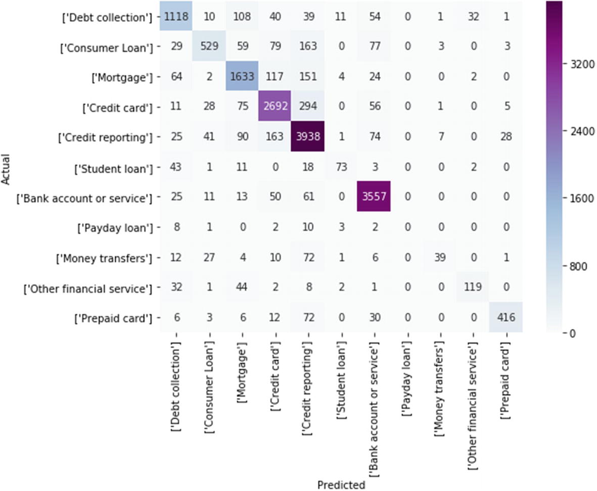
Step 1-4 Data understanding

Let’s analyze the columns:
Data.dtypes
date_received                   object
product                         object
sub_product                     object
issue                           object
sub_issue                       object
consumer_complaint_narrative    object
company_public_response         object
company                         object
state                           object
zipcode                         object
tags                            object
consumer_consent_provided       object
submitted_via                   object
date_sent_to_company            object
company_response_to_consumer    object
timely_response                 object
consumer_disputed?              object
complaint_id                     int64
# Selecting required columns and rows
Data = Data[['product', 'consumer_complaint_narrative']]
Data = Data[pd.notnull(Data['consumer_complaint_narrative'])]
# See top 5 rows
Data.head()
                product           consumer_complaint_narrative
190126  Debt collection    XXXX has claimed I owe them {$27.00} for XXXX ...
190135    Consumer Loan    Due to inconsistencies in the amount owed that...
190155          Mortgage    In XX/XX/XXXX my wages that I earned at my job...
190207          Mortgage    I have an open and current mortgage with Chase...
190208         Mortgage    XXXX was submitted XX/XX/XXXX. At the time I s...
# Factorizing the category column
Data['category_id'] = Data['product'].factorize()[0]
Data.head()
                product    consumer_complaint_narrative   
190126  Debt collection    XXXX has claimed I owe them {$27.00} for XXXX ...
190135    Consumer Loan    Due to inconsistencies in the amount owed that...
        category_id
190126            0
190135            1
# Check the distriution of complaints by category
Data.groupby('product').consumer_complaint_narrative.count()
product
Bank account or service    5711
Consumer Loan              3678
Credit card                7929
Credit reporting           12526
Debt collection            17552
Money transfers              666
Mortgage                   14919
Other financial service      110
Payday loan                  726
Prepaid card                 861
Student loan                2128
# Lets plot it and see
fig = plt.figure(figsize=(8,6))
Data.groupby('product').consumer_complaint_narrative.count().plot.bar(ylim=0)
plt.show()
../images/475440_1_En_5_Chapter/475440_1_En_5_Figa_HTML.jpg

Debt collection and Mortgage have the highest number of complaints registered.

Step 1-5 Splitting the data

Split the data into train and validation:
train_x, valid_x, train_y, valid_y = model_selection.train_test_split(Data['consumer_complaint_narrative'], Data['product'])

Step 1-6 Feature engineering using TF-IDF

Create TF-IDF vectors as we discussed in Chapter 3. Here we consider maximum features to be 5000.
encoder = preprocessing.LabelEncoder()
train_y = encoder.fit_transform(train_y)
valid_y = encoder.fit_transform(valid_y)
tfidf_vect = TfidfVectorizer(analyzer='word', token_pattern=r'w{1,}', max_features=5000)
tfidf_vect.fit(Data['consumer_complaint_narrative'])
xtrain_tfidf =  tfidf_vect.transform(train_x)
xvalid_tfidf =  tfidf_vect.transform(valid_x)

Step 1-7 Model building and evaluation

Suppose we are building a linear classifier on word-level TF-IDF vectors. We are using default hyper parameters for the classifier. Parameters can be changed like C, max_iter, or solver to obtain better results.
model = linear_model.LogisticRegression().fit(xtrain_tfidf, train_y)
# Model summary
LogisticRegression(C=1.0, class_weight=None, dual=False, fit_intercept=True,
          intercept_scaling=1, max_iter=100, multi_class="ovr", n_jobs=1,
          penalty='l2', random_state=None, solver="liblinear", tol=0.0001,
          verbose=0, warm_start=False)
# Checking accuracy
accuracy = metrics.accuracy_score(model.predict(xvalid_tfidf), valid_y)
print ("Accuracy: ", accuracy)
Accuracy:  0.845048497186
# Classification report
print(metrics.classification_report(valid_y, model.predict(xvalid_tfidf),target_names=Data['product'].unique()))
                        precision    recall  f1-score   support
        Debt collection    0.81      0.79      0.80       1414
          Consumer Loan    0.81      0.56      0.66        942
               Mortgage    0.80      0.82      0.81       1997
            Credit card    0.85      0.85      0.85       3162
       Credit reporting    0.82      0.90      0.86       4367
           Student loan    0.77      0.48      0.59        151
  Bank account or service    0.92      0.96      0.94       3717
            Payday loan    0.00      0.00      0.00         26
        Money transfers    0.76      0.23      0.35        172
Other financial service    0.77      0.57      0.65        209
           Prepaid card    0.92      0.76      0.83        545
            avg / total    0.84      0.85      0.84      16702
#confusion matrix
conf_mat = confusion_matrix(valid_y, model.predict(xvalid_tfidf))
# Vizualizing confusion matrix
category_id_df = Data[['product', 'category_id']].drop_duplicates().sort_values('category_id')
category_to_id = dict(category_id_df.values)
id_to_category = dict(category_id_df[['category_id', 'product']].values)
fig, ax = plt.subplots(figsize=(8,6))
sns.heatmap(conf_mat, annot=True, fmt="d", cmap="BuPu",
            xticklabels=category_id_df[['product']].values, yticklabels=category_id_df[['product']].values)
plt.ylabel('Actual')
plt.xlabel('Predicted')
plt.show()
../images/475440_1_En_5_Chapter/475440_1_En_5_Figb_HTML.jpg
The accuracy of 85% is good for a baseline model. Precision and recall look pretty good across the categories except for “Payday loan.” If you look for Payload loan, most of the wrong predictions are Debt collection and Credit card, which might be because of the smaller number of samples in that category. It also sounds like it’s a subcategory of a credit card. We can add these samples to any other group to make the model more stable. Let’s see what prediction looks like for one example.
# Prediction example
texts = ["This company refuses to provide me verification and validation of debt"+ "per my right under the FDCPA. I do not believe this debt is mine."]
text_features = tfidf_vect.transform(texts)
predictions = model.predict(text_features)
print(texts)
print("  - Predicted as: '{}'".format(id_to_category[predictions[0]]))
Result :
['This company refuses to provide me verification and validation of debtper my right under the FDCPA. I do not believe this debt is mine.']
  - Predicted as: 'Credit reporting'
To increase the accuracy, we can do the following things:
  • Reiterate the process with different algorithms like Random Forest, SVM, GBM, Neural Networks, Naive Bayes.

  • Deep learning techniques like RNN and LSTM (will be discussed in next chapter) can also be used.

  • In each of these algorithms, there are so many parameters to be tuned to get better results. It can be easily done through Grid search, which will basically try out all possible combinations and give the best out.

Recipe 5-2. Implementing Sentiment Analysis

In this recipe, we are going to implement, end to end, one of the popular NLP industrial applications – Sentiment Analysis. It is very important from a business standpoint to understand how customer feedback is on the products/services they offer to improvise on the products/service for customer satisfaction.

Problem

We want to implement sentiment analysis.

Solution

The simplest way to do this by using the TextBlob or vaderSentiment library. Since we have used TextBlob previously, now let us use vader.

How It Works

Let’s follow the steps in this section to implement sentiment analysis on the business problem.

Step 2-1 Understanding/defining business problem

Understand how products are doing in the market. How are customers reacting to a particular product? What is the consumer’s sentiment across products? Many more questions like these can be answered using sentiment analysis.

Step 2-2 Identifying potential data sources, collection, and understanding

We have a dataset for Amazon food reviews. Let’s use that data and extract insight out of it. You can download the data from the link below:
https://www.kaggle.com/snap/amazon-fine-food-reviews
# Import necessary libraries
import numpy as np
import pandas as pd
import matplotlib.pyplot as plt
%matplotlib inline
#Read the data
df = pd.read_csv('Reviews.csv')
# Look at the top 5 rows of the data
df.head(5)
#output
../images/475440_1_En_5_Chapter/475440_1_En_5_Figc_HTML.jpg
# Understand the data types of the columns
df.info()
# Output
Data columns (total 10 columns):
Id                        5 non-null int64
ProductId                 5 non-null object
UserId                    5 non-null object
ProfileName               5 non-null object
HelpfulnessNumerator      5 non-null int64
HelpfulnessDenominator    5 non-null int64
Score                     5 non-null int64
Time                      5 non-null int64
Summary                   5 non-null object
Text                      5 non-null object
dtypes: int64(5), object(5)
# Looking at the summary of the reviews.
df.Summary.head(5)
# Output
0    Good Quality Dog Food
1        Not as Advertised
2    "Delight" says it all
3           Cough Medicine
4              Great taffy
# Looking at the description of the reviews
df.Text.head(5)
#output
0    I have bought several of the Vitality canned d...
1    Product arrived labeled as Jumbo Salted Peanut...
2    This is a confection that has been around a fe...
3    If you are looking for the secret ingredient i...
4    Great taffy at a great price.  There was a wid...

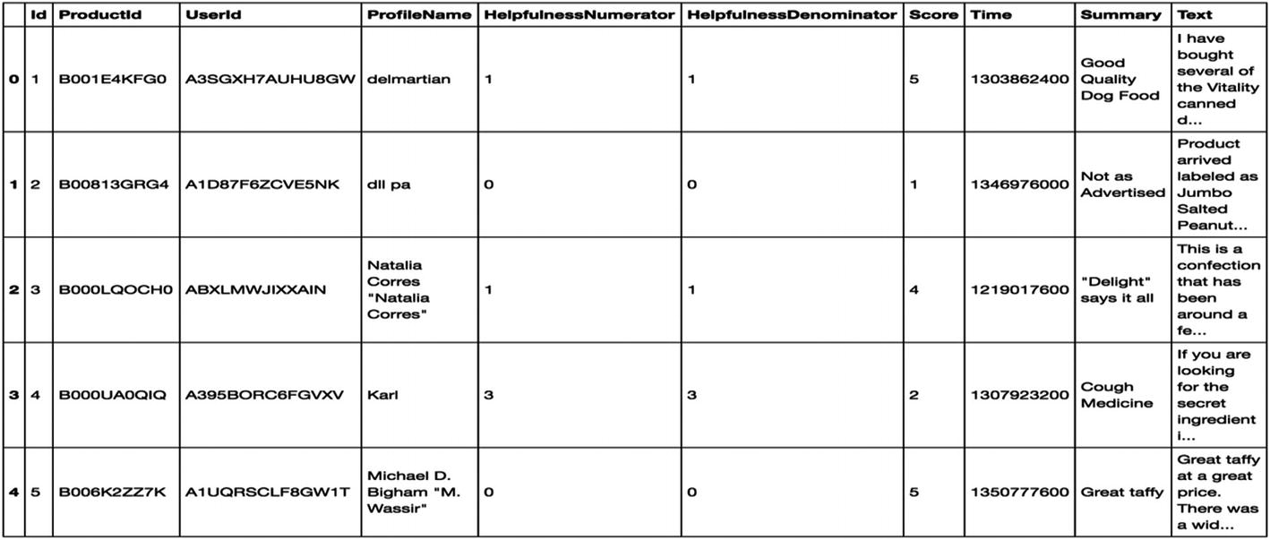
Step 2-3 Text preprocessing

We all know the importance of this step. Let us perform a preprocessing task as discussed in Chapter 2.
# Import libraries
from nltk.corpus import stopwords
from textblob import TextBlob
from textblob import Word
# Lower casing and removing punctuations
df['Text'] = df['Text'].apply(lambda x: " ".join(x.lower() for x in x.split()))
df['Text'] = df['Text'].str.replace('[^ws]',")
df.Text.head(5)
# Output
0    i have bought several of the vitality canned d...
1    product arrived labeled as jumbo salted peanut...
2    this is a confection that has been around a fe...
3    if you are looking for the secret ingredient i...
4    great taffy at a great price there was a wide ...
# Removal of stop words
stop = stopwords.words('english')
df['Text'] = df['Text'].apply(lambda x: " ".join(x for x in x.split() if x not in stop))
df.Text.head(5)
# Output
0    bought several vitality canned dog food produc...
1    product arrived labeled jumbo salted peanutsth...
2    confection around centuries light pillowy citr...
3    looking secret ingredient robitussin believe f...
4    great taffy great price wide assortment yummy ...
# Spelling correction
df['Text'] = df['Text'].apply(lambda x: str(TextBlob(x).correct()))
df.Text.head(5)
# Output
0    bought several vitality canned dog food produc...
1    product arrived labelled lumbo halted peanutst...
2    connection around centuries light pillow citie...
3    looking secret ingredient robitussin believe f...
4    great staff great price wide assortment mummy ...
# Lemmatization
df['Text'] = df['Text'].apply(lambda x: " ".join([Word(word).lemmatize() for word in x.split()]))
df.Text.head(5)
# Output
0    bought several vitality canned dog food produc...
1    product arrived labelled lumbo halted peanutst...
2    connection around century light pillow city ge...
3    looking secret ingredient robitussin believe f...
4    great staff great price wide assortment mummy ...

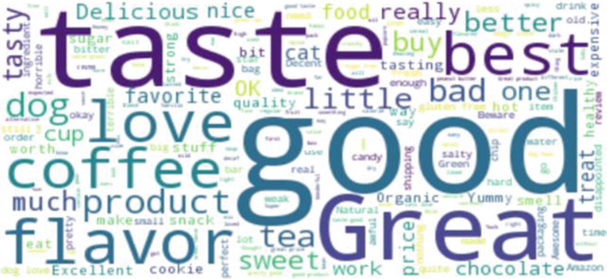
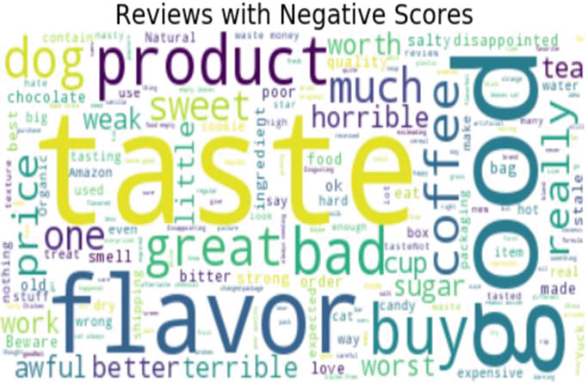
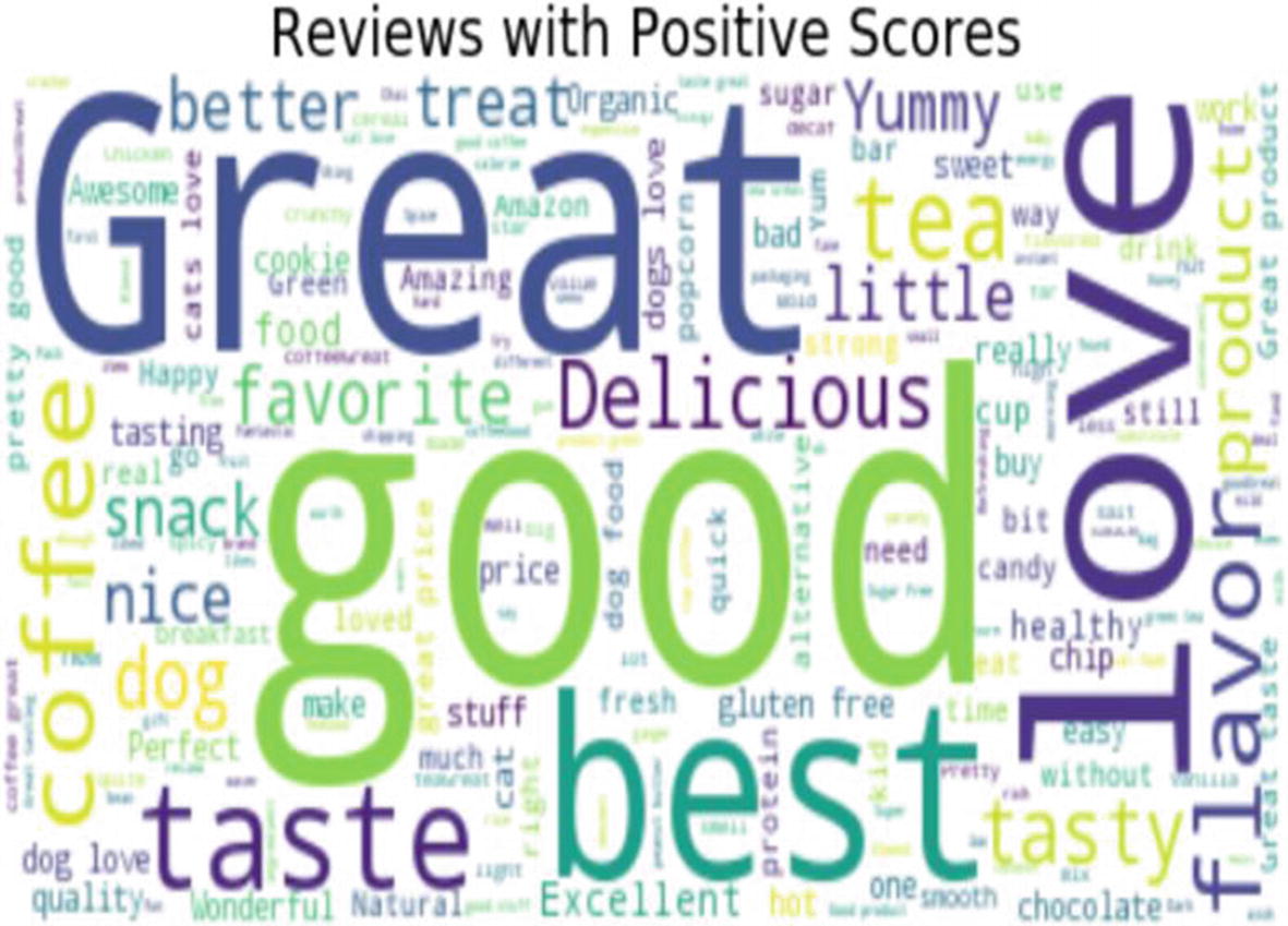
Step 2-4 Exploratory data analysis

This step is not connected anywhere in predicting sentiments; what we are trying to do here is to dig deeper into the data and understand it.
# Create a new data frame "reviews" to perform exploratory data analysis upon that
reviews = df
# Dropping null values
reviews.dropna(inplace=True)
# The histogram reveals this dataset is highly unbalanced towards high rating.
reviews.Score.hist(bins=5,grid=False)
plt.show()
print(reviews.groupby('Score').count().Id)
../images/475440_1_En_5_Chapter/475440_1_En_5_Figd_HTML.jpg
# To make it balanced data, we sampled each score by the lowest n-count from above. (i.e. 29743 reviews scored as '2')
score_1 = reviews[reviews['Score'] == 1].sample(n=29743)
score_2 = reviews[reviews['Score'] == 2].sample(n=29743)
score_3 = reviews[reviews['Score'] == 3].sample(n=29743)
score_4 = reviews[reviews['Score'] == 4].sample(n=29743)
score_5 = reviews[reviews['Score'] == 5].sample(n=29743)
# Here we recreate a 'balanced' dataset.
reviews_sample = pd.concat([score_1,score_2,score_3,score_4,score_5],axis=0)
reviews_sample.reset_index(drop=True,inplace=True)
You can use this dataset if you are training your own sentiment classifier from scratch. And to do this. you can follow the same steps as in text classification (Recipe 5-1). Here our target variable would be positive, negative, and neutral created using score.
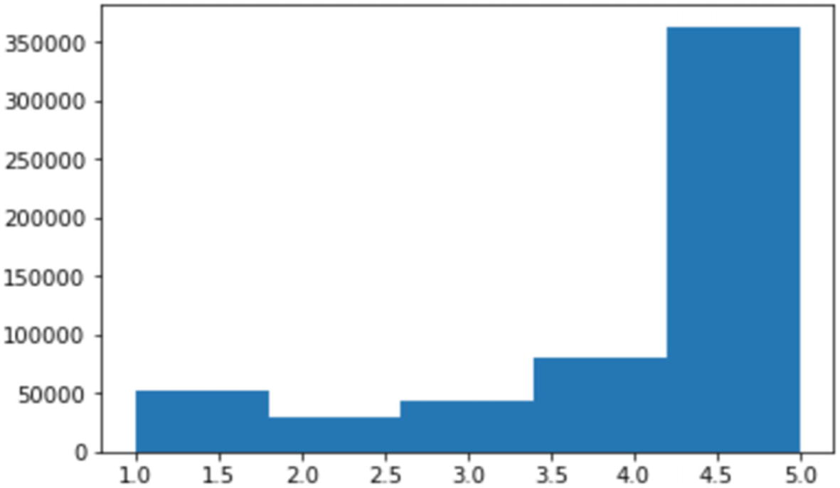
  • Score <= 2: Negative

  • Score = 3: Neutral

  • Score > =4: Positive

Having said that, let’s get back to our exploratory data analysis.
# Printing count by 'Score' to check dataset is now balanced.
print(reviews_sample.groupby('Score').count().Id)
# Output
Score
1    29743
2    29743
3    29743
4    29743
5    29743
# Let's build a word cloud looking at the 'Summary'  text
from wordcloud import WordCloud
from wordcloud import STOPWORDS
# Wordcloud function's input needs to be a single string of text.
# Here I'm concatenating all Summaries into a single string.
# similarly you can build for Text column
reviews_str = reviews_sample.Summary.str.cat()
wordcloud = WordCloud(background_color='white').generate(reviews_str)
plt.figure(figsize=(10,10))
plt.imshow(wordcloud,interpolation='bilinear')
plt.axis("off")
plt.show()
../images/475440_1_En_5_Chapter/475440_1_En_5_Fige_HTML.jpg
# Now let's split the data into Negative (Score is 1 or 2) and Positive (4 or #5) Reviews.
negative_reviews = reviews_sample[reviews_sample['Score'].isin([1,2]) ]
positive_reviews = reviews_sample[reviews_sample['Score'].isin([4,5]) ]
# Transform to single string
negative_reviews_str = negative_reviews.Summary.str.cat()
positive_reviews_str = positive_reviews.Summary.str.cat()
# Create wordclouds
wordcloud_negative = WordCloud(background_color='white').generate(negative_reviews_str)
wordcloud_positive = WordCloud(background_color='white').generate(positive_reviews_str)
# Plot
fig = plt.figure(figsize=(10,10))
ax1 = fig.add_subplot(211)
ax1.imshow(wordcloud_negative,interpolation='bilinear')
ax1.axis("off")
ax1.set_title('Reviews with Negative Scores',fontsize=20)
../images/475440_1_En_5_Chapter/475440_1_En_5_Figf_HTML.jpg
ax2 = fig.add_subplot(212)
ax2.imshow(wordcloud_positive,interpolation='bilinear')
ax2.axis("off")
ax2.set_title('Reviews with Positive Scores',fontsize=20)
plt.show()
#output
../images/475440_1_En_5_Chapter/475440_1_En_5_Figg_HTML.jpg

Step 2-5 Feature engineering

This step is not required as we are not building the model from scratch; rather we are using the pretrained model from the library vaderSentiment.

If you want to build the model from scratch, you can leverage the above positive and negative classes created while exploring as a target variable and then training the model. You can follow the same steps as text classification explained in Recipe 5-1 to build a sentiment classifier from scratch.

Step 2-6 Sentiment scores

Sentiment Analysis: Pretrained model takes the input from the text description and outputs the sentiment score ranging from -1 to +1 for each sentence.
#Importing required libraries
import pandas as pd
import numpy as np
import matplotlib.pyplot as plt
%matplotlib inline
import seaborn as sns
import re
import os
import sys
import ast
plt.style.use('fivethirtyeight')
# Function for getting the sentiment
cp = sns.color_palette()
from vaderSentiment.vaderSentiment import SentimentIntensityAnalyzer
analyzer = SentimentIntensityAnalyzer()
# Generating sentiment for all the sentence present in the dataset
emptyline=[]
for row in df['Text']:
    vs=analyzer.polarity_scores(row)
    emptyline.append(vs)
# Creating new dataframe with sentiments    
df_sentiments=pd.DataFrame(emptyline)
df_sentiments.head(5)
# Output
      compound    neg    neu    pos
0     0.9413      0.000  0.503  0.497
1    -0.5719      0.258  0.644  0.099
2     0.8031      0.133  0.599  0.268
3     0.4404      0.000  0.854  0.146
4     0.9186      0.000  0.455  0.545
# Merging the sentiments back to reviews dataframe
df_c = pd.concat([df.reset_index(drop=True), d], axis=1)
df_c.head(3)
#output sample
../images/475440_1_En_5_Chapter/475440_1_En_5_Figh_HTML.jpg
# Convert scores into positive and negetive sentiments using some threshold
df_c['Sentiment'] = np.where(df_c['compound'] >= 0 , 'Positive', 'Negative')
df_c.head(5)
#output sample
../images/475440_1_En_5_Chapter/475440_1_En_5_Figi_HTML.jpg

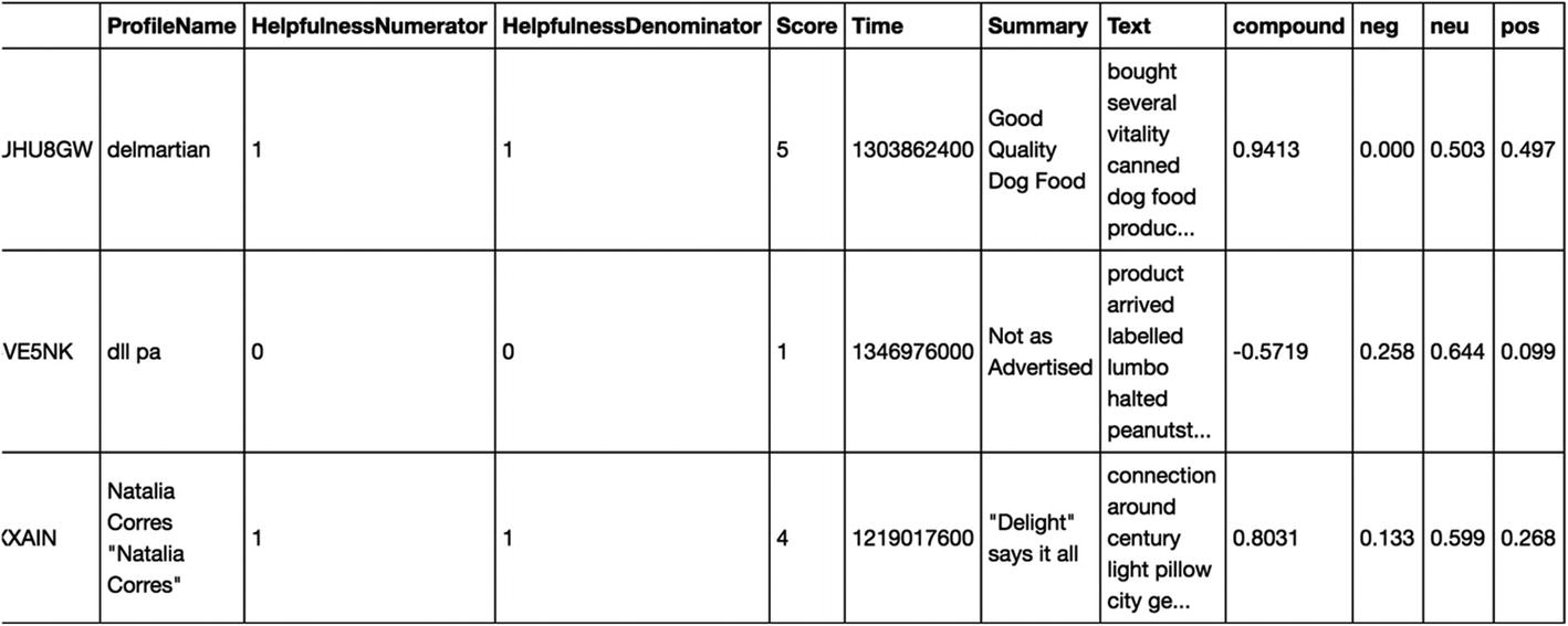
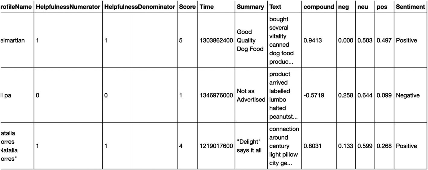
Step 2-7 Business insights

Let’s see how the overall sentiment is using the sentiment we generated.
result=df_c['Sentiment'].value_counts()
result.plot(kind='bar', rot=0,color='br');
../images/475440_1_En_5_Chapter/475440_1_En_5_Figj_HTML.jpg

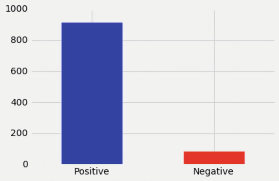
We just took a sample of 1000 reviews and completed sentiment analysis. If you look, more than 900 (>90%) reviews are positive, which is really good for any business.

We can also group by-products, that is, sentiments by-products to understand the high-level customer feedback against products.
#Sample code snippet
result=df_c.groupby('ProductId')['Sentiment'].value_counts().unstack()
result[['Negative','Positive']].plot(kind='bar', rot=0,color='rb')

Similarly, we can analyze sentiments by month using the time column and many other such attributes.

Recipe 5-3. Applying Text Similarity Functions

This recipe covers data stitching using text similarity.

Problem

We will have multiple tables in the database, and sometimes there won’t be a common “ID” or “KEY” to join them – scenarios like the following:
  • Customer information scattered across multiple tables and systems.

  • No global key to link them all together.

  • A lot of variations in names and addresses.

Solution

This can be solved by applying text similarity functions on the demographic’s columns like the first name, last name, address, etc. And based on the similarity score on a few common columns, we can decide either the record pair is a match or not a match.

How It Works

Let’s follow the steps in this section to link the records.

Technical challenge:
  • Huge records that need to be linked/stitched/deduplicated.

  • Records come from various systems with differing schemas.

There is no global key or customer id to merge. There are two possible scenarios of data stitching or linking records:
  • Multiple records of the same customer at the same table, and you want to dedupe.

  • Records of same customers from multiple tables need to be merged.

For Recipe 3-A, let’s solve scenario 1 that is deduplication and as a part of Recipe 3-B, let’s solve scenario 2 that is record linkage from multiple tables.

Deduplication in the same table

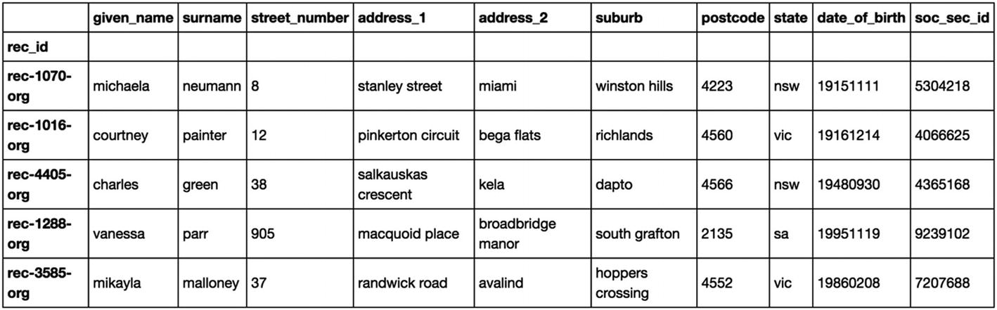
Step 3A-1 Read and understand the data
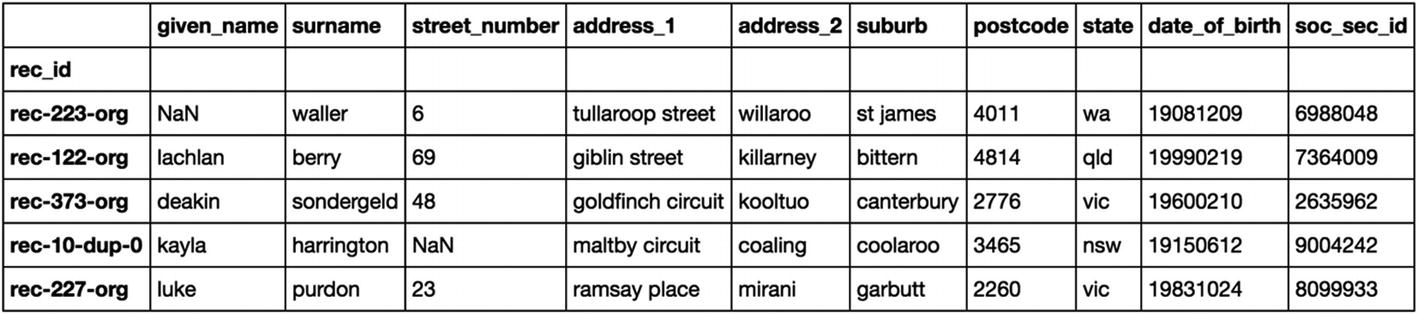
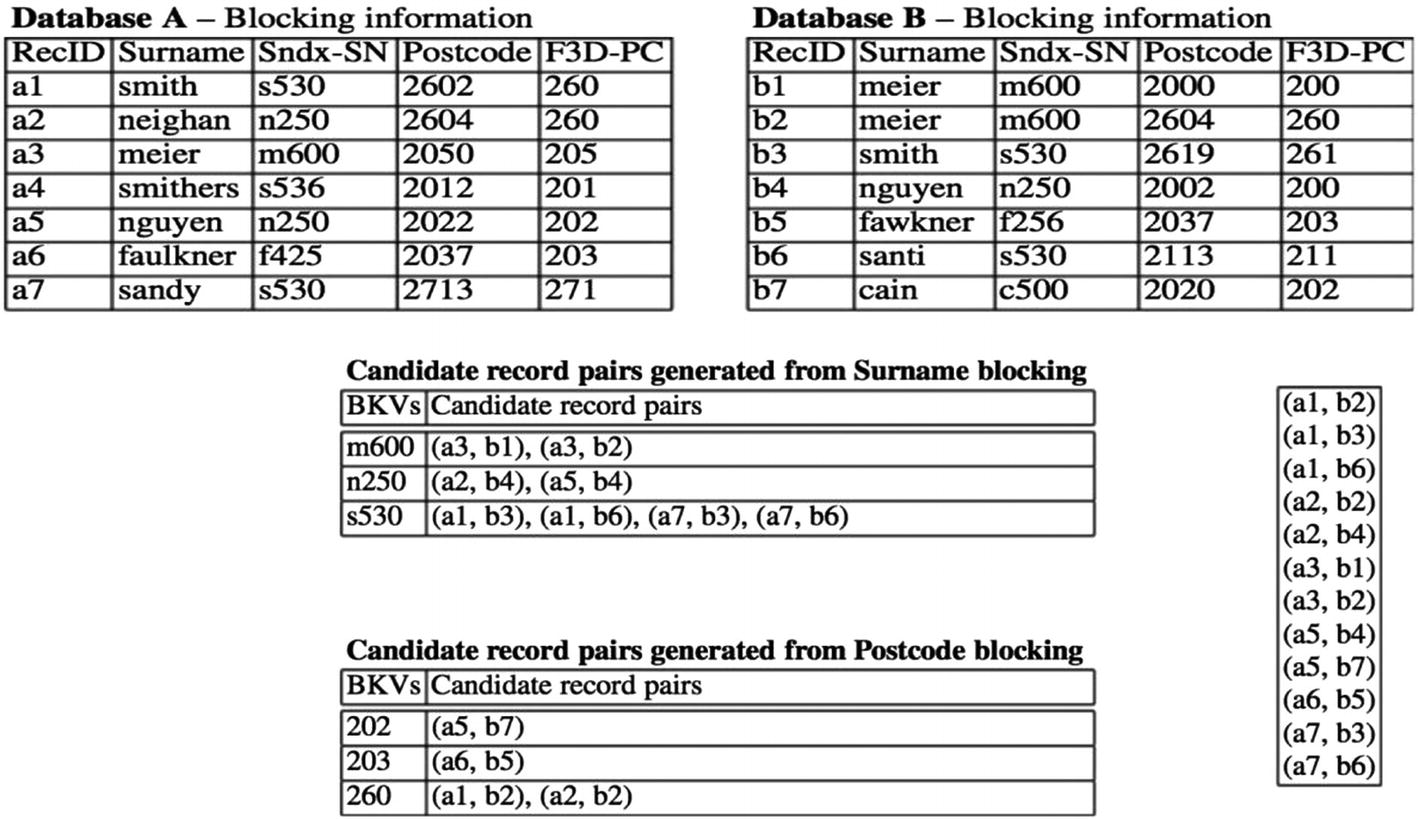
We need the data first:
# Import package
!pip install recordlinkage
import recordlinkage
#For this demo let us use the inbuilt dataset from recordlinkage library
#import data set
from recordlinkage.datasets import load_febrl1
#create a dataframe - dfa
dfA = load_febrl1()
dfA.head()
#output
../images/475440_1_En_5_Chapter/475440_1_En_5_Figk_HTML.jpg
Step 3A-2 Blocking

Here we reduce the comparison window and create record pairs.

Why?
  • Suppose there are huge records say, 100M records means (100M choose 2) ≈ 10^16 possible pairs

  • Need heuristic to quickly cut that 10^16 down without losing many matches

This can be accomplished by extracting a “blocking key” How? Example:
  • Record: first name: John, last name: Roberts, address: 20 Main St Plainville MA 01111

  • Blocking key: first name - John

  • Will be paired with: John Ray … 011

  • Won’t be paired with: Frank Sinatra … 07030

  • Generate pairs only for records in the same block

Below is the blocking example at a glance: here blocking is done on the “Sndx-SN,” column which is nothing but the Soundex value of the surname column as discussed in the previous chapter.

../images/475440_1_En_5_Chapter/475440_1_En_5_Figl_HTML.jpg
There are many advanced blocking techniques, also, like the following:
  • Standard blocking
    • Single column

    • Multiple columns

  • Sorted neighborhood

  • Q-gram: fuzzy blocking

  • LSH

  • Canopy clustering

This can be a new topic altogether, but for now, let’s build the pairs using the first name as the blocking index.
indexer = recordlinkage.BlockIndex(on='given_name')
pairs = indexer.index(dfA)
print (len(pairs))
#output
2082
Step 3A-3 Similarity matching and scoring

Here we compute the similarity scores on the columns like given name, surname, and address between the record pairs generated in the previous step. For columns like date of birth, suburb, and state, we are using the exact match as it is important for this column to possess exact records.

We are using jarowinkler, but you can use any of the other similarity measures discussed in Chapter 4.
# This cell can take some time to compute.
compare_cl = recordlinkage.Compare()
compare_cl.string('given_name', 'given_name',method='jarowinkler', label="given_name")
compare_cl.string('surname', 'surname', method="jarowinkler", label="surname")
compare_cl.exact('date_of_birth', 'date_of_birth', label="date_of_birth")
compare_cl.exact('suburb', 'suburb', label="suburb")
compare_cl.exact('state', 'state', label="state")
compare_cl.string('address_1', 'address_1',method='jarowinkler', label="address_1")
features = compare_cl.compute(pairs, dfA)
features.sample(5)
#output
../images/475440_1_En_5_Chapter/475440_1_En_5_Figm_HTML.jpg

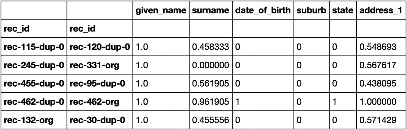
So here record “rec-115-dup-0” is compared with “rec-120-dup-0.” Since their first name (blocking column) is matching, similarity scores are calculated on the common columns for these pairs.

Step 3A-4 Predicting records match or do not match using ECM – classifier
Here is an unsupervised learning method to calculate the probability that the records match.
# select all the features except for given_name since its our blocking key
features1 = features[['suburb','state','surname','date_of_birth','address_1']]
# Unsupervised learning – probabilistic
ecm = recordlinkage.ECMClassifier()
result_ecm = ecm.learn((features1).astype(int),return_type = 'series')
result_ecm
#output
rec_id rec_id
rec-122-org rec-183-dup-0 0
 rec-248-org 0
 rec-469-org 0
 rec-74-org 0
 rec-183-org 0
 rec-360-dup-0 0
 rec-248-dup-0 0
 rec-469-dup-0 0
rec-183-dup-0 rec-248-org 0
 rec-469-org 0
 rec-74-org 0
 rec-183-org 1
 rec-360-dup-0 0
 rec-248-dup-0 0
 rec-469-dup-0 0
rec-248-org rec-469-org 0
 rec-74-org 0
 rec-360-dup-0 0
 rec-469-dup-0 0
rec-122-dup-0 rec-122-org 1
 rec-183-dup-0 0
 rec-248-org 0
 rec-469-org 0
 rec-74-org 0
 rec-183-org 0
 rec-360-dup-0 0
 rec-248-dup-0 0
 rec-469-dup-0 0
rec-469-org rec-74-org 0
rec-183-org rec-248-org 0
 ..
rec-208-dup-0 rec-208-org 1
rec-363-dup-0 rec-363-org 1
rec-265-dup-0 rec-265-org 1
rec-315-dup-0 rec-315-org 1
rec-410-dup-0 rec-410-org 1
rec-290-org rec-93-org 0
rec-460-dup-0 rec-460-org 1
rec-499-dup-0 rec-499-org 1
rec-11-dup-0 rec-11-org 1
rec-97-dup-0 rec-97-org 1
rec-213-dup-0 rec-421-dup-0 0
rec-349-dup-0 rec-376-dup-0 0
rec-371-dup-0 rec-371-org 1
rec-129-dup-0 rec-129-org 1
rec-462-dup-0 rec-462-org 1
rec-328-dup-0 rec-328-org 1
rec-308-dup-0 rec-308-org 1
rec-272-org rec-308-dup-0 0
 rec-308-org 0
rec-5-dup-0 rec-5-org 1
rec-407-dup-0 rec-407-org 1
rec-367-dup-0 rec-367-org 1
rec-103-dup-0 rec-103-org 1
rec-195-dup-0 rec-195-org 1
rec-184-dup-0 rec-184-org 1
rec-252-dup-0 rec-252-org 1
rec-48-dup-0 rec-48-org 1
rec-298-dup-0 rec-298-org 1
rec-282-dup-0 rec-282-org 1
rec-327-org rec-411-org 0

The output clearly shows that “rec-183-dup-0” matches “rec-183-org” and can be linked to one global_id. What we have done so far is deduplication: identifying multiple records of the same users from the individual table.

Records of same customers from multiple tables

Next, let us look at how we can solve this problem if records are in multiple tables without unique ids to merge with.

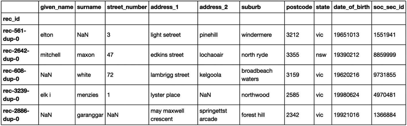
Step 3B-1 Read and understand the data
Let us use the built-in dataset from the recordlinkage library:
from recordlinkage.datasets import load_febrl4
dfA, dfB = load_febrl4()
dfA.head()
#output
../images/475440_1_En_5_Chapter/475440_1_En_5_Fign_HTML.jpg
dfB.head()
#output
../images/475440_1_En_5_Chapter/475440_1_En_5_Figo_HTML.jpg
Step 3B-2 Blocking – to reduce the comparison window and creating record pairs
This is the same as explained previously, considering the given_name as a blocking index:
indexer = recordlinkage.BlockIndex(on='given_name')
pairs = indexer.index(dfA, dfB)
Step 3B-3 Similarity matching
The explanation remains the same.
compare_cl = recordlinkage.Compare()
compare_cl.string('given_name', 'given_name',method='jarowinkler', label="given_name")
compare_cl.string('surname', 'surname', method="jarowinkler", label="surname")
compare_cl.exact('date_of_birth', 'date_of_birth', label="date_of_birth")
compare_cl.exact('suburb', 'suburb', label="suburb")
compare_cl.exact('state', 'state', label="state")
compare_cl.string('address_1', 'address_1',method='jarowinkler', label="address_1")
features = compare_cl.compute(pairs, dfA, dfB)
features.head(10)
#output
../images/475440_1_En_5_Chapter/475440_1_En_5_Figp_HTML.jpg

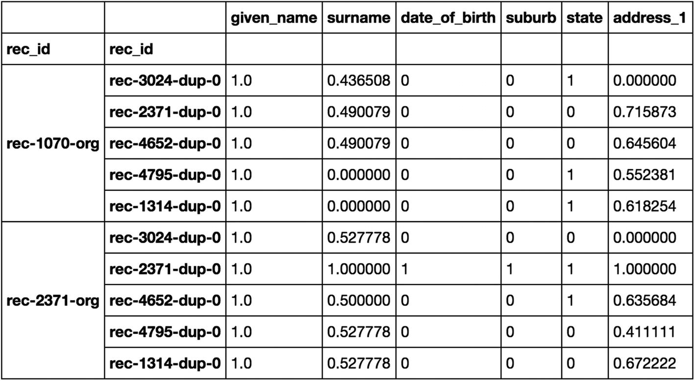
So here record “rec-1070-org” is compared with “rec-3024-dup-0,” “rec-2371-dup-0,” “rec-4652-dup-0,” “rec-4795-dup-0,” and “rec-1314-dup-0, since their first name (blocking column) is matching and similarity scores are calculated on the common columns for these pairs.

Step 3B-4 Predicting records match or do not match using ECM – classifier
Here is an unsupervised learning method to calculate the probability that the record is a match.
# select all the features except for given_name since its our blocking key
features1 = features[['suburb','state','surname','date_of_birth','address_1']]
# unsupervised learning - probablistic
ecm = recordlinkage.ECMClassifier()
result_ecm = ecm.learn((features1).astype(int),return_type = 'series')
result_ecm
#output sample
rec_id        rec_id
rec-1070-org  rec-3024-dup-0    0
              rec-2371-dup-0    0
              rec-4652-dup-0    0
              rec-4795-dup-0    0
              rec-1314-dup-0    0
rec-2371-org  rec-3024-dup-0    0
              rec-2371-dup-0    1
              rec-4652-dup-0    0
              rec-4795-dup-0    0
              rec-1314-dup-0    0
rec-3582-org  rec-3024-dup-0    0
              rec-2371-dup-0    0
              rec-4652-dup-0    0
              rec-4795-dup-0    0
              rec-1314-dup-0    0
rec-3024-org  rec-3024-dup-0    1
              rec-2371-dup-0    0
              rec-4652-dup-0    0
              rec-4795-dup-0    0
              rec-1314-dup-0    0
rec-4652-org  rec-3024-dup-0    0
              rec-2371-dup-0    0
              rec-4652-dup-0    1
              rec-4795-dup-0    0
              rec-1314-dup-0    0
rec-4795-org  rec-3024-dup-0    0
              rec-2371-dup-0    0
              rec-4652-dup-0    0
              rec-4795-dup-0    1
              rec-1314-dup-0    0
                               ..
rec-2820-org  rec-2820-dup-0    1
              rec-991-dup-0     0
rec-1984-org  rec-1984-dup-0    1
rec-1662-org  rec-1984-dup-0    0
rec-4415-org  rec-1984-dup-0    0
rec-1920-org  rec-1920-dup-0    1
rec-303-org   rec-303-dup-0     1
rec-1915-org  rec-1915-dup-0    1
rec-4739-org  rec-4739-dup-0    1
              rec-4865-dup-0    0
rec-681-org   rec-4276-dup-0    0
rec-4603-org  rec-4848-dup-0    0
              rec-4603-dup-0    1
rec-3122-org  rec-4848-dup-0    0
              rec-4603-dup-0    0
rec-3711-org  rec-3711-dup-0    1
rec-4912-org  rec-4912-dup-0    1
rec-664-org   rec-664-dup-0     1
              rec-1311-dup-0    0
rec-4031-org  rec-4031-dup-0    1
rec-1413-org  rec-1413-dup-0    1
rec-735-org   rec-735-dup-0     1
rec-1361-org  rec-1361-dup-0    1
rec-3090-org  rec-3090-dup-0    1
rec-2571-org  rec-2571-dup-0    1
rec-4528-org  rec-4528-dup-0    1
rec-4887-org  rec-4887-dup-0    1
rec-4350-org  rec-4350-dup-0    1
rec-4569-org  rec-4569-dup-0    1
rec-3125-org  rec-3125-dup-0    1

The output clearly shows that “rec-122-dup-0” matches “rec-122-org” and can be linked to one global_id.

In this way, you can create a data lake consisting of a unique global id and consistent data across tables and also perform any kind of statistical analysis.

Recipe 5-4. Summarizing Text Data

If you just look around, there are lots of articles and books available. Let’s assume you want to learn a concept in NLP and if you Google it, you will find an article. You like the content of the article, but it’s too long to read it one more time. You want to basically summarize the article and save it somewhere so that you can read it later.

Well, NLP has a solution for that. Text summarization will help us do that. You don’t have to read the full article or book every time.

Problem

Text summarization of article/document using different algorithms in Python.

Solution

Text summarization is the process of making large documents into smaller ones without losing the context, which eventually saves readers time. This can be done using different techniques like the following:
  • TextRank: A graph-based ranking algorithm

  • Feature-based text summarization

  • LexRank: TF-IDF with a graph-based algorithm

  • Topic based

  • Using sentence embeddings

  • Encoder-Decoder Model: Deep learning techniques

How It Works

We will explore the first 2 approaches in this recipe and see how it works.

Method 4-1 TextRank

TextRank is the graph-based ranking algorithm for NLP. It is basically inspired by PageRank, which is used in the Google search engine but particularly designed for text. It will extract the topics, create nodes out of them, and capture the relation between nodes to summarize the text.

Let’s see how to do it using the Python package Gensim. “Summarize” is the function used.

Before that, let’s import the notes. Let’s say your article is Wikipedia for the topic of Natural language processing.
# Import BeautifulSoup and urllib libraries to fetch data from Wikipedia.
from bs4 import BeautifulSoup
from urllib.request import urlopen
# Function to get data from Wikipedia
def get_only_text(url):
 page = urlopen(url)
 soup = BeautifulSoup(page)
 text = ' '.join(map(lambda p: p.text, soup.find_all('p')))
 print (text)
 return soup.title.text, text
# Mention the Wikipedia url
url="https://en.wikipedia.org/wiki/Natural_language_processing"
# Call the function created above
text = get_only_text(url)
# Count the number of letters
len(".join(text))
Result:
Out[74]: 8519
# Lets see first 1000 letters from the text
text[:1000]
Result :
Out[72]: '('Natural language processing - Wikipedia', 'Natural language processing (NLP) is an area of computer science and artificial intelligence concerned with the interactions between computers and human (natural) languages, in particular how to program computers to process and analyze large amounts of natural language\xa0data.\n Challenges in natural language processing frequently involve speech recognition, natural language understanding, and natural language generation.\n The history of natural language processing generally started in the 1950s, although work can be found from earlier periods.\nIn 1950, Alan Turing published an article titled "Intelligence" which proposed what is now called the Turing test as a criterion of intelligence.\n The Georgetown experiment in 1954 involved fully automatic translation of more than sixty Russian sentences into English. The authors claimed that within three or five years, machine translation would be a solved problem.[2]  However, real progress was '
# Import summarize from gensim
from gensim.summarization.summarizer import summarize
from gensim.summarization import keywords
# Convert text to string format
text = str(text)
#Summarize the text with ratio 0.1 (10% of the total words.)
summarize(text, ratio=0.1)
Result:
Out[77]: 'However, part-of-speech tagging introduced the use of hidden Markov models to natural language processing, and increasingly, research has focused on statistical models, which make soft, probabilistic decisions based on attaching real-valued weights to the features making up the input data. Such models are generally more robust when given unfamiliar input, especially input that contains errors (as is very common for real-world data), and produce more reliable results when integrated into a larger system comprising multiple subtasks.\n Many of the notable early successes occurred in the field of machine translation, due especially to work at IBM Research, where successively more complicated statistical models were developed.'
That’s it. The generated summary is as simple as that. If you read this summary and whole article, it's close enough. But still, there is a lot of room for improvement.
#keywords
print(keywords(text, ratio=0.1))
Result:
learning
learn
languages
process
systems
worlds
world
real
natural language processing
research
researched
results
result
data
statistical
hand
generation
generally
generic
general
generated
tasks
task
large
human
intelligence
input
called
calling
calls
produced
produce
produces
producing
possibly
possible
corpora
base
based

Method 4-2 Feature-based text summarization

Your feature-based text summarization methods will extract a feature from the sentence and check the importance to rank it. Position, length, term frequency, named entity, and many other features are used to calculate the score.

Luhn’s Algorithm is one of the feature-based algorithms, and we will see how to implement it using the sumy library.
# Install sumy
!pip install sumy
# Import the packages
from sumy.parsers.html import HtmlParser
from sumy.parsers.plaintext import PlaintextParser
from sumy.nlp.tokenizers import Tokenizer
from sumy.summarizers.lsa import LsaSummarizer
from sumy.nlp.stemmers import Stemmer
from sumy.utils import get_stop_words
from sumy.summarizers.luhn import LuhnSummarizer
# Extracting and summarizing
LANGUAGE = "english"
SENTENCES_COUNT = 10
url="https://en.wikipedia.org/wiki/Natural_language_processing"
parser = HtmlParser.from_url(url, Tokenizer(LANGUAGE))
summarizer = LsaSummarizer()
summarizer = LsaSummarizer(Stemmer(LANGUAGE))
summarizer.stop_words = get_stop_words(LANGUAGE)
for sentence in summarizer(parser.document, SENTENCES_COUNT):
    print(sentence)
Result :
[2] However, real progress was much slower, and after the ALPAC report in 1966, which found that ten-year-long research had failed to fulfill the expectations, funding for machine translation was dramatically reduced.
However, there is an enormous amount of non-annotated data available (including, among other things, the entire content of the World Wide Web ), which can often make up for the inferior results if the algorithm used has a low enough time complexity to be practical , which some such as Chinese Whispers do.
Since the so-called "statistical revolution"
in the late 1980s and mid 1990s, much natural language processing research has relied heavily on machine learning .
Increasingly, however, research has focused on statistical models , which make soft, probabilistic decisions based on attaching real-valued weights to each input feature.
Natural language understanding Convert chunks of text into more formal representations such as first-order logic structures that are easier for computer programs to manipulate.
[18] ^ Implementing an online help desk system based on conversational agent Authors: Alisa Kongthon, Chatchawal Sangkeettrakarn, Sarawoot Kongyoung and Choochart Haruechaiyasak.
[ self-published source ] ^ Chomskyan linguistics encourages the investigation of " corner cases " that stress the limits of its theoretical models (comparable to pathological phenomena in mathematics), typically created using thought experiments , rather than the systematic investigation of typical phenomena that occur in real-world data, as is the case in corpus linguistics .
^ Antonio Di Marco - Roberto Navigili, "Clustering and Diversifying Web Search Results with Graph Based Word Sense Induction" , 2013 Goldberg, Yoav (2016).
Scripts, plans, goals, and understanding: An inquiry into human knowledge structures ^ Kishorjit, N., Vidya Raj RK., Nirmal Y., and Sivaji B.
^ PASCAL Recognizing Textual Entailment Challenge (RTE-7) https://tac.nist.gov//2011/RTE/ ^ Yi, Chucai; Tian, Yingli (2012), "Assistive Text Reading from Complex Background for Blind Persons" , Camera-Based Document Analysis and Recognition , Springer Berlin Heidelberg, pp.

Problem solved. Now you don’t have to read the whole notes; just read the summary whenever we are running low on time.

We can use many of the deep learning techniques to get better accuracy and better results like the Encoder-Decoder Model. We will see how to do that in the next chapter.

Recipe 5-5. Clustering Documents

Document clustering, also called text clustering, is a cluster analysis on textual documents. One of the typical usages would be document management.

Problem

Clustering or grouping the documents based on the patterns and similarities.

Solution

Document clustering yet again includes similar steps , so let’s have a look at them:
  1. 1.

    Tokenization

     
  2. 2.

    Stemming and lemmatization

     
  3. 3.

    Removing stop words and punctuation

     
  4. 4.

    Computing term frequencies or TF-IDF

     
  5. 5.

    Clustering: K-means/Hierarchical; we can then use any of the clustering algorithms to cluster different documents based on the features we have generated

     
  6. 6.

    Evaluation and visualization: Finally, the clustering results can be visualized by plotting the clusters into a two-dimensional space


How It Works

Step 5-1 Import data and libraries

Here are the libraries, then the data:
!pip install mpld3
import numpy as np
import pandas as pd
import nltk
from nltk.stem.snowball import SnowballStemmer
from bs4 import BeautifulSoup
import re
import os
import codecs
from sklearn import feature_extraction
import mpld3
from sklearn.metrics.pairwise import cosine_similarity
import os
import matplotlib.pyplot as plt
import matplotlib as mpl
from sklearn.manifold import MDS
#Lets use the same complaint dataset we use for classification
Data = pd.read_csv("/Consumer_Complaints.csv",encoding='latin-1')
#selecting required columns and rows
Data = Data[['consumer_complaint_narrative']]
Data = Data[pd.notnull(Data['consumer_complaint_narrative'])]
# lets do the clustering for just 200 documents . Its easier to interpret.
Data_sample=Data.sample(200)

Step 5-2 Preprocessing and TF-IDF feature engineering

Now we preprocess it:
# Remove unwanted symbol
Data_sample['consumer_complaint_narrative'] = Data_sample['consumer_complaint_narrative'].str.replace('XXXX',")
# Convert dataframe to list
complaints = Data_sample['consumer_complaint_narrative'].tolist()
# create the rank of documents – we will use it later
ranks = []
for i in range(1, len(complaints)+1):
    ranks.append(i)
# Stop Words
stopwords = nltk.corpus.stopwords.words('english')
# Load 'stemmer'
stemmer = SnowballStemmer("english")
# Functions for sentence tokenizer, to remove numeric tokens and raw #punctuation
def tokenize_and_stem(text):
    tokens = [word for sent in nltk.sent_tokenize(text) for word in nltk.word_tokenize(sent)]
    filtered_tokens = []
    for token in tokens:
        if re.search('[a-zA-Z]', token):
            filtered_tokens.append(token)
    stems = [stemmer.stem(t) for t in filtered_tokens]
    return stems
def tokenize_only(text):
    tokens = [word.lower() for sent in nltk.sent_tokenize(text) for word in nltk.word_tokenize(sent)]
    filtered_tokens = []
    for token in tokens:
        if re.search('[a-zA-Z]', token):
            filtered_tokens.append(token)
    return filtered_tokens
from sklearn.feature_extraction.text import TfidfVectorizer
# tfidf vectorizer
tfidf_vectorizer = TfidfVectorizer(max_df=0.8, max_features=200000,
                                 min_df=0.2, stop_words="english",
                                 use_idf=True, tokenizer=tokenize_and_stem, ngram_range=(1,3))
#fit the vectorizer to data
tfidf_matrix = tfidf_vectorizer.fit_transform(complaints)
terms = tfidf_vectorizer.get_feature_names()
print(tfidf_matrix.shape)
(200, 30)

Step 5-3 Clustering using K-means

Let’s start the clustering:
#Import Kmeans
from sklearn.cluster import KMeans
# Define number of clusters
num_clusters = 6
#Running clustering algorithm
km = KMeans(n_clusters=num_clusters)
km.fit(tfidf_matrix)
#final clusters
clusters = km.labels_.tolist()
complaints_data = { 'rank': ranks, 'complaints': complaints, 'cluster': clusters }
frame = pd.DataFrame(complaints_data, index = [clusters] , columns = ['rank', 'cluster'])
#number of docs per cluster
frame['cluster'].value_counts()
0 42
1 37
5 36
3 36
2 27
4 22

Step 5-4 Identify cluster behavior

Identify which are the top 5 words that are nearest to the cluster centroid.
totalvocab_stemmed = []
totalvocab_tokenized = []
for i in complaints:
    allwords_stemmed = tokenize_and_stem(i)
    totalvocab_stemmed.extend(allwords_stemmed)
    allwords_tokenized = tokenize_only(i)
    totalvocab_tokenized.extend(allwords_tokenized)
vocab_frame = pd.DataFrame({'words': totalvocab_tokenized}, index = totalvocab_stemmed)
#sort cluster centers by proximity to centroid
order_centroids = km.cluster_centers_.argsort()[:, ::-1]
for i in range(num_clusters):
    print("Cluster %d words:" % i, end=")
    for ind in order_centroids[i, :6]:
        print(' %s' % vocab_frame.ix[terms[ind].split(' ')].values.tolist()[0][0].encode('utf-8', 'ignore'), end=',')
    print()
Cluster 0 words: b'needs', b'time', b'bank', b'information', b'told'
Cluster 1 words: b'account', b'bank', b'credit', b'time', b'months'
Cluster 2 words: b'debt', b'collection', b'number', b'credit', b"n't"
Cluster 3 words: b'report', b'credit', b'credit', b'account', b'information'
Cluster 4 words: b'loan', b'payments', b'pay', b'months', b'state'
Cluster 5 words: b'payments', b'pay', b'told', b'did', b'credit'

Step 5-5 Plot the clusters on a 2D graph

Finally, we plot the clusters:
#Similarity
similarity_distance = 1 - cosine_similarity(tfidf_matrix)
# Convert two components as we're plotting points in a two-dimensional plane
mds = MDS(n_components=2, dissimilarity="precomputed", random_state=1)
pos = mds.fit_transform(similarity_distance)  # shape (n_components, n_samples)
xs, ys = pos[:, 0], pos[:, 1]
#Set up colors per clusters using a dict
cluster_colors = {0: '#1b9e77', 1: '#d95f02', 2: '#7570b3', 3: '#e7298a', 4: '#66a61e', 5: '#D2691E'}
#set up cluster names using a dict
cluster_names = {0: 'property, based, assist',
                 1: 'business, card',
                 2: 'authorized, approved, believe',
                 3: 'agreement, application,business',
                 4: 'closed, applied, additional',
                 5: 'applied, card'}
# Finally plot it
%matplotlib inline
#Create data frame that has the result of the MDS and the cluster
df = pd.DataFrame(dict(x=xs, y=ys, label=clusters))
groups = df.groupby('label')
# Set up plot
fig, ax = plt.subplots(figsize=(17, 9)) # set size
for name, group in groups:
    ax.plot(group.x, group.y, marker="o", linestyle=", ms=20,
            label=cluster_names[name], color=cluster_colors[name],
            mec='none')
    ax.set_aspect('auto')
    ax.tick_params(
        axis= 'x',
        which='both',
        bottom='off',
        top='off',
        labelbottom='off')
    ax.tick_params(
        axis= 'y',
        which='both',
        left='off',
        top='off',
        labelleft='off')
ax.legend(numpoints=1)
plt.show()
../images/475440_1_En_5_Chapter/475440_1_En_5_Figq_HTML.jpg

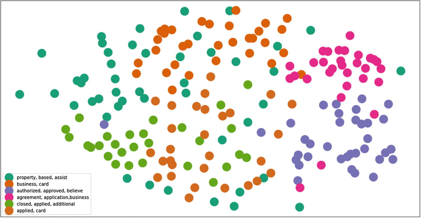
That’s it. We have clustered 200 complaints into 6 groups using K-means clustering. It basically clusters similar kinds of complaints to 6 buckets using TF-IDF. We can also use the word embeddings and solve this to achieve better clusters. 2D graphs provide a good look into the cluster's behavior and if we look, we will see that the same color dots (docs) are located closer to each other.

Recipe 5-6. NLP in a Search Engine

In this recipe, we are going to discuss what it takes to build a search engine from an NLP standpoint. Implementation of the same is beyond the scope of this book.

Problem

You want to know the architecture and NLP pipeline to build a search engine.

Solution

Figure 5-1 shows the whole process. Each step is explained in the “How It Works” section.
../images/475440_1_En_5_Chapter/475440_1_En_5_Fig1_HTML.jpg
Figure 5-1

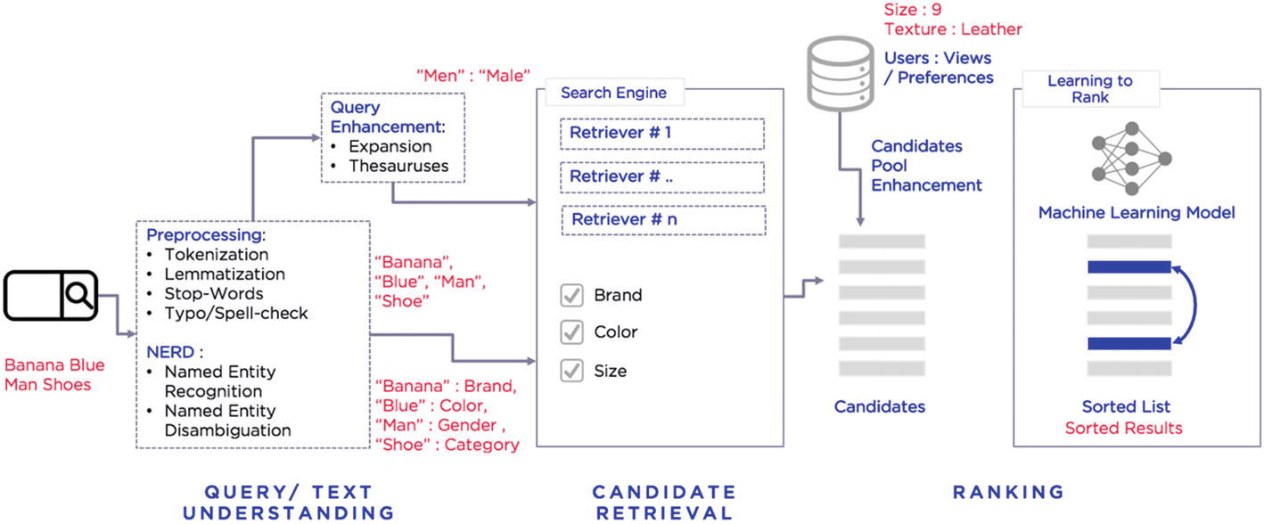
The NLP process in a search engine

How It Works

Let’s follow and understand the above architecture step by step in this section to build the search engine from an NLP standpoint.

Step 6-1 Preprocessing

Whenever the user enters the search query, it is passed on to the NLP preprocessing pipeline:
  1. 1.

    Removal of noise and stop words

     
  2. 2.

    Tokenization

     
  3. 3.

    Stemming

     
  4. 4.

    Lemmatization


Step 6-2 The entity extraction model

Output from the above pipeline is fed into the entity extraction model . We can build the customized entity recognition model by using any of the libraries like StanfordNER or NLTK.

Or you can build an entity recognition model from scratch using conditional random fields or Markov models.

For example, suppose we are building a search engine for an e-commerce giant. Below are entities that we can train the model on:
  • Gender

  • Color

  • Brand

  • Product Category

  • Product Type

  • Price

  • Size

Also, we can build named entity disambiguation using deep learning frameworks like RNN and LSTM. This is very important for the entities extractor to understand the content in which the entities are used. For example, pink can be a color or a brand. NED helps in such disambiguation.

NERD Model building steps:
  • Data cleaning and preprocessing

  • Training NER Model

  • Testing and Validation

  • Deployment

Ways to train/build NERD model :
  • Named Entity Recognition and Disambiguation

  • Stanford NER with customization

  • Recurrent Neural Network (RNN) – LSTM (Long Short-Term Memory) to use context for disambiguation

  • Joint Named Entity Recognition and Disambiguation

Step 6-3 Query enhancement/expansion

It is very important to understand the possible synonyms of the entities to make sure search results do not miss out on potential relevance. Say, for example, men’s shoes can also be called as male shoes, men’s sports shoes, men’s formal shoes, men’s loafers, men’s sneakers.

Use locally-trained word embedding (using Word2Vec / GloVe Model ) to achieve this.

Step 6-4 Use a search platform

Search platforms such as Solr or Elastic Search have major features that include full-text search hit highlighting, faceted search, real-time indexing, dynamic clustering, and database integration. This is not related to NLP; as an end-to-end application point of view, we have just given an introduction of what this is.

Step 6-5 Learning to rank

Once the search results are fetched from Solr or Elastic Search, they should be ranked based on the user preferences using the past behaviors.

..................Content has been hidden....................

You can't read the all page of ebook, please click here login for view all page.
Reset
18.191.223.208