
Recipe 1. One Hot encoding
Recipe 2. Count vectorizer
Recipe 3. N-grams
Recipe 4. Co-occurrence matrix
Recipe 5. Hash vectorizer
Recipe 6. Term Frequency-Inverse Document Frequency (TF-IDF)
Recipe 7. Word embedding
Recipe 8. Implementing fastText
Now that all the text preprocessing steps are discussed, let’s explore feature engineering, the foundation for Natural Language Processing. As we already know, machines or algorithms cannot understand the characters/words or sentences, they can only take numbers as input that also includes binaries. But the inherent nature of text data is unstructured and noisy, which makes it impossible to interact with machines.
The procedure of converting raw text data into machine understandable format (numbers) is called feature engineering of text data. Machine learning and deep learning algorithms’ performance and accuracy is fundamentally dependent on the type of feature engineering technique used.
In this chapter, we will discuss different types of feature engineering methods along with some state-of-the-art techniques; their functionalities, advantages, disadvantages; and examples for each. All of these will make you realize the importance of feature engineering.
Recipe 3-1. Converting Text to Features Using One Hot Encoding
The traditional method used for feature engineering is One Hot encoding. If anyone knows the basics of machine learning, One Hot encoding is something they should have come across for sure at some point of time or maybe most of the time. It is a process of converting categorical variables into features or columns and coding one or zero for the presence of that particular category. We are going to use the same logic here, and the number of features is going to be the number of total tokens present in the whole corpus.
Problem
You want to convert text to feature using One Hot encoding.
Solution
I | love | NLP | is | future | |
|---|---|---|---|---|---|
I love NLP | 1 | 1 | 1 | 0 | 0 |
NLP is future | 0 | 0 | 1 | 1 | 1 |
How It Works
There are so many functions to generate One Hot encoding. We will take one function and discuss it in depth.
Step 1-1 Store the text in a variable
Step 1-2 Execute below function on the text data
Output has 4 features since the number of distinct words present in the input was 4.
Recipe 3-2. Converting Text to Features Using Count Vectorizing
The approach in Recipe 3-1 has a disadvantage. It does not take the frequency of the word occurring into consideration. If a particular word is appearing multiple times, there is a chance of missing the information if it is not included in the analysis. A count vectorizer will solve that problem.
In this recipe, we will see the other method of converting text to feature, which is a count vectorizer.
Problem
How do we convert text to feature using a count vectorizer?
Solution
Count vectorizer is almost similar to One Hot encoding. The only difference is instead of checking whether the particular word is present or not, it will count the words that are present in the document.
I | love | NLP | is | future | will | learn | in | 2month | |
|---|---|---|---|---|---|---|---|---|---|
I love NLP and I will learn NLP in 2 months | 2 | 1 | 2 | 0 | 0 | 1 | 1 | 1 | 1 |
NLP is future | 0 | 0 | 1 | 1 | 1 | 0 | 0 | 0 | 0 |
How It Works
The fifth token nlp has appeared twice in the document.
Recipe 3-3. Generating N-grams
If you observe the above methods, each word is considered as a feature. There is a drawback to this method.
It does not consider the previous and the next words, to see if that would give a proper and complete meaning to the words.
For example: consider the word “not bad.” If this is split into individual words, then it will lose out on conveying “good” – which is what this word actually means.
As we saw, we might lose potential information or insight because a lot of words make sense once they are put together. This problem can be solved by N-grams.
Unigrams are the unique words present in the sentence.
Bigram is the combination of 2 words.
Trigram is 3 words and so on.
For example,
“I am learning NLP”
Unigrams: “I”, “am”, “ learning”, “NLP”
Bigrams: “I am”, “am learning”, “learning NLP”
Trigrams: “I am learning”, “am learning NLP”
Problem
Generate the N-grams for the given sentence.
Solution
There are a lot of packages that will generate the N-grams. The one that is mostly used is TextBlob.
How It Works
Following are the steps.
Step 3-1 Generating N-grams using TextBlob
If we observe, we have 3 lists with 2 words at an instance.
Step 3-2 Bigram-based features for a document
The output has features with bigrams, and for our example, the count is one for all the tokens.
Recipe 3-4. Generating Co-occurrence Matrix
Let’s discuss one more method of feature engineering called a co-occurrence matrix.
Problem
Understand and generate a co-occurrence matrix.
Solution
A co-occurrence matrix is like a count vectorizer where it counts the occurrence of the words together, instead of individual words.
How It Works
Let’s see how to generate these kinds of matrixes using nltk, bigrams, and some basic Python coding skills.
Step 4-1 Import the necessary libraries
Step 4-2 Create function for co-occurrence matrix
Step 4-3 Generate co-occurrence matrix
If you observe, “I,” “love,” and “is,” nlp” has appeared together twice, and a few other words appeared only once.
Recipe 3-5. Hash Vectorizing
A count vectorizer and co-occurrence matrix have one limitation though. In these methods, the vocabulary can become very large and cause memory/computation issues.
One of the ways to solve this problem is a Hash Vectorizer.
Problem
Understand and generate a Hash Vectorizer.
Solution
Hash Vectorizer is memory efficient and instead of storing the tokens as strings, the vectorizer applies the hashing trick to encode them as numerical indexes. The downside is that it’s one way and once vectorized, the features cannot be retrieved.
How It Works
Let’s take an example and see how to do it using sklearn.
Step 5-1 Import the necessary libraries and create document
Step 5-2 Generate hash vectorizer matrix
Recipe 3-6. Converting Text to Features Using TF-IDF
Let’s say a particular word is appearing in all the documents of the corpus, then it will achieve higher importance in our previous methods. That’s bad for our analysis.
The whole idea of having TF-IDF is to reflect on how important a word is to a document in a collection, and hence normalizing words appeared frequently in all the documents.
Problem
Text to feature using TF-IDF.
Solution
Term frequency (TF): Term frequency is simply the ratio of the count of a word present in a sentence, to the length of the sentence.
TF is basically capturing the importance of the word irrespective of the length of the document. For example, a word with the frequency of 3 with the length of sentence being 10 is not the same as when the word length of sentence is 100 words. It should get more importance in the first scenario; that is what TF does.
Inverse Document Frequency (IDF): IDF of each word is the log of the ratio of the total number of rows to the number of rows in a particular document in which that word is present.
IDF = log(N/n), where N is the total number of rows and n is the number of rows in which the word was present.
IDF will measure the rareness of a term. Words like “a,” and “the” show up in all the documents of the corpus, but rare words will not be there in all the documents. So, if a word is appearing in almost all documents, then that word is of no use to us since it is not helping to classify or in information retrieval. IDF will nullify this problem.
TF-IDF is the simple product of TF and IDF so that both of the drawbacks are addressed, which makes predictions and information retrieval relevant.
How It Works
Let's look at the following steps.
Step 6-1 Read the text data
Step 6-2 Creating the Features
If you observe, “the” is appearing in all the 3 documents and it does not add much value, and hence the vector value is 1, which is less than all the other vector representations of the tokens.
All these methods or techniques we have looked into so far are based on frequency and hence called frequency-based embeddings or features. And in the next recipe, let us look at prediction-based embeddings, typically called word embeddings.
Recipe 3-7. Implementing Word Embeddings
This recipe assumes that you have a working knowledge of how a neural network works and the mechanisms by which weights in the neural network are updated. If new to a Neural Network (NN), it is suggested that you go through Chapter 6 to gain a basic understanding of how NN works.
Even though all previous methods solve most of the problems, once we get into more complicated problems where we want to capture the semantic relation between the words, these methods fail to perform.
- All these techniques fail to capture the context and meaning of the words. All the methods discussed so far basically depend on the appearance or frequency of the words. But we need to look at how to capture the context or semantic relations: that is, how frequently the words are appearing close by.
- a.
I am eating an apple.
- b.
I am using apple.
- a.
For a problem like a document classification (book classification in the library) , a document is really huge and there are a humongous number of tokens generated. In these scenarios, your number of features can get out of control (wherein) thus hampering the accuracy and performance.
A machine/algorithm can match two documents/texts and say whether they are same or not. But how do we make machines tell you about cricket or Virat Kohli when you search for MS Dhoni? How do you make a machine understand that “Apple” in “Apple is a tasty fruit” is a fruit that can be eaten and not a company?
The answer to the above questions lies in creating a representation for words that capture their meanings, semantic relationships, and the different types of contexts they are used in.
The above challenges are addressed by Word Embeddings.
Word embedding is the feature learning technique where words from the vocabulary are mapped to vectors of real numbers capturing the contextual hierarchy.
Words | Vectors | ||||
|---|---|---|---|---|---|
text | 0.36 | 0.36 | -0.43 | 0.36 | |
idea | -0.56 | -0.56 | 0.72 | -0.56 | |
word | 0.35 | -0.43 | 0.12 | 0.72 | |
encode | 0.19 | 0.19 | 0.19 | 0.43 | |
document | -0.43 | 0.19 | -0.43 | 0.43 | |
grams | 0.72 | -0.43 | 0.72 | 0.12 | |
process | 0.43 | 0.72 | 0.43 | 0.43 | |
feature | 0.12 | 0.45 | 0.12 | 0.87 | |
Problem
You want to implement word embeddings.
Solution
Word embeddings are prediction based, and they use shallow neural networks to train the model that will lead to learning the weight and using them as a vector representation.
word2vec : word2vec is the deep learning Google framework to train word embeddings. It will use all the words of the whole corpus and predict the nearby words. It will create a vector for all the words present in the corpus in a way so that the context is captured. It also outperforms any other methodologies in the space of word similarity and word analogies.
Skip-Gram
Continuous Bag of Words (CBOW)

How It Works
The above figure shows the architecture of the CBOW and skip-gram algorithms used to build word embeddings. Let us see how these models work in detail.
Skip-Gram
The skip-gram model (Mikolov et al., 2013)1 is used to predict the probabilities of a word given the context of word or words.
Let us take a small sentence and understand how it actually works. Each sentence will generate a target word and context, which are the words nearby. The number of words to be considered around the target variable is called the window size. The table below shows all the possible target and context variables for window size 2. Window size needs to be selected based on data and the resources at your disposal. The larger the window size, the higher the computing power.
Target word | Context | |
|---|---|---|
I love NLP | I | love, NLP |
I love NLP and | love | love, NLP, and |
I love NLP and I will learn | NLP | I, love, and, I |
… | … | … |
in 2 months | month | in, 2 |
Since it takes a lot of text and computing power, let us go ahead and take sample data and build a skip-gram model.
We get an error saying the word doesn’t exist because this word was not there in our input training data. This is the reason we need to train the algorithm on as much data possible so that we do not miss out on words.
Result:
Continuous Bag of Words (CBOW)
Result:
But to train these models, it requires a huge amount of computing power. So, let us go ahead and use Google’s pre-trained model, which has been trained with over 100 billion words.
Download the model from the below path and keep it in your local storage:
https://drive.google.com/file/d/0B7XkCwpI5KDYNlNUTTlSS21pQmM/edit
If you add ‘woman’ and ‘king’ and minus man, it is predicting queen as output with 77% confidence. Isn’t this amazing?

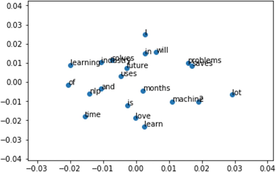
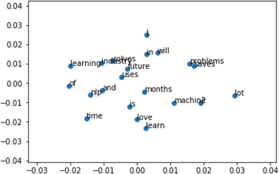
Let’s have a look at few of the interesting examples using T – SNE plot for word embeddings.
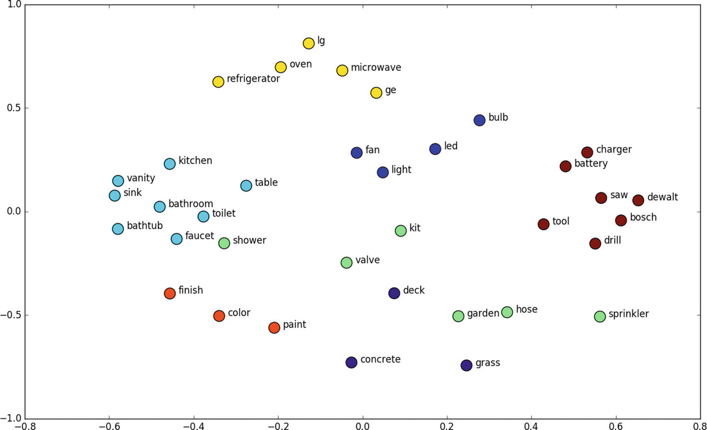
Above is the word embedding’s output representation of home interiors and exteriors. If you clearly observe, all the words related to electric fittings are near to each other; similarly, words related to bathroom fittings are near to each other, and so on. This is the beauty of word embeddings.
Recipe 3-8 Implementing fastText
fastText is another deep learning framework developed by Facebook to capture context and meaning.
Problem
How to implement fastText in Python.
Solution
fastText is the improvised version of word2vec. word2vec basically considers words to build the representation. But fastText takes each character while computing the representation of the word.
How It Works
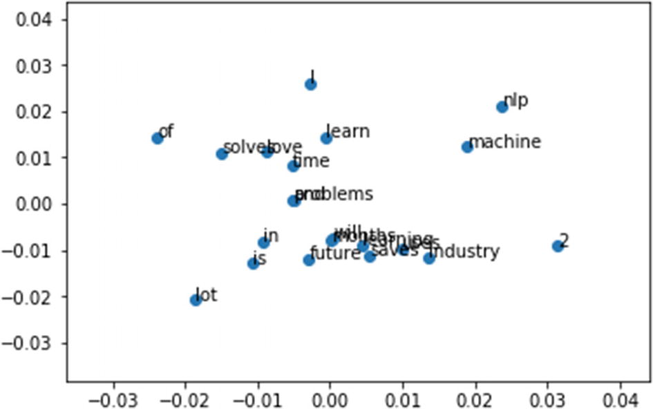
The figure above shows the embedding representation for fastText. If you observe closely, the words “love” and “solve” are close together in fastText but in your skip-gram and CBOW, “love” and “learn” are near to each other. This is an effect of character-level embeddings.
We hope that by now you are familiar and comfortable with processing the natural language. Now that data is cleaned and features are created, let’s jump into building some applications around it that solves the business problem.