© Akshay Kulkarni and Adarsha Shivananda 2019
Akshay Kulkarni and Adarsha ShivanandaNatural Language Processing Recipeshttps://doi.org/10.1007/978-1-4842-4267-4_6

6. Deep Learning for NLP

Akshay Kulkarni1  and Adarsha Shivananda1
(1)
Bangalore, Karnataka, India
 
In this chapter, we will implement deep learning for NLP:
  • Recipe 1. Information retrieval using deep learning

  • Recipe 2. Text classification using CNN, RNN, LSTM

  • Recipe 3. Predicting the next word/sequence of words using LSTM for Emails

Introduction to Deep Learning

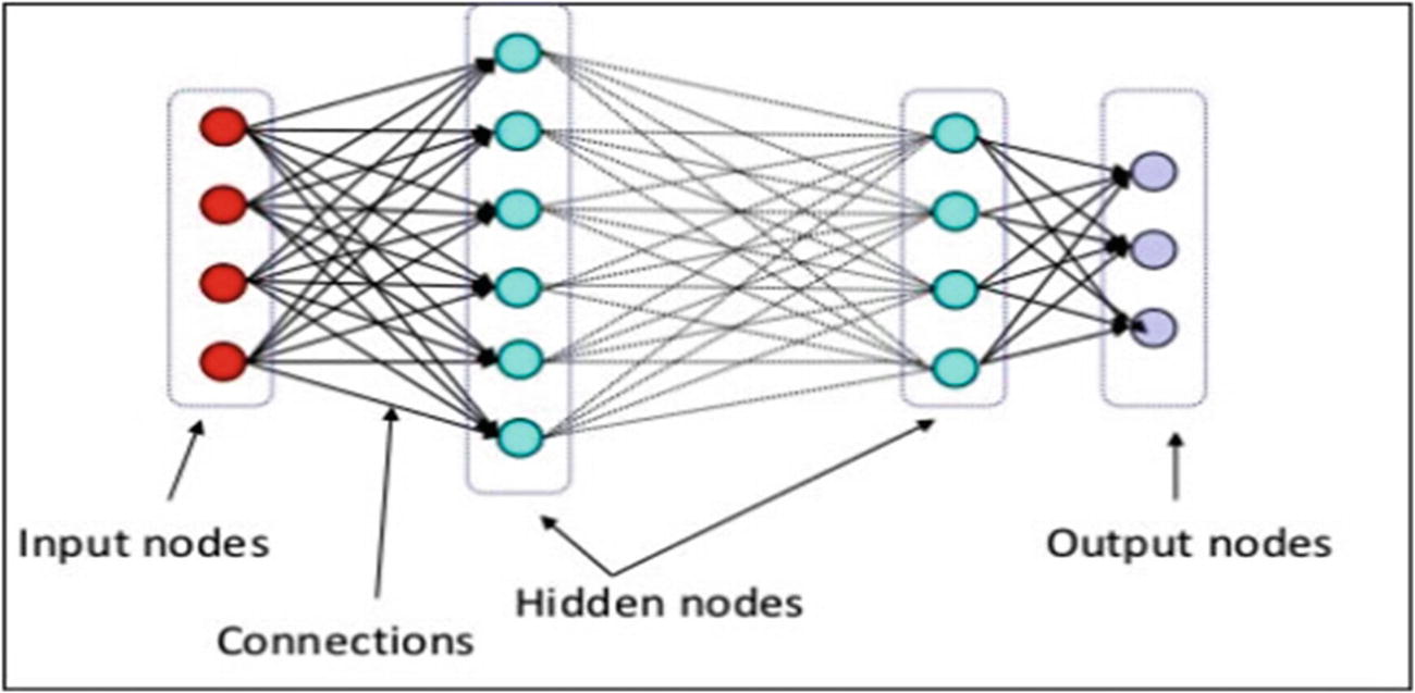
Deep learning is a subfield of machine learning that is inspired by the function of the brain. Just like how neurons are interconnected in the brain, neural networks also work the same. Each neuron takes input, does some kind of manipulation within the neuron, and produces an output that is closer to the expected output (in the case of labeled data).

What happens within the neuron is what we are interested in: to get to the most accurate results. In very simple words, it’s giving weight to every input and generating a function to accumulate all these weights and pass it onto the next layer, which can be the output layer eventually.

The network has 3 components:
  • Input layer

  • Hidden layer/layers

  • Output layer

../images/475440_1_En_6_Chapter/475440_1_En_6_Figa_HTML.jpg
The functions can be of different types based on the problem or the data. These are also called activation functions. Below are the types.
  • Linear Activation functions: A linear neuron takes a linear combination of the weighted inputs; and the output can take any value between -infinity to infinity.

  • Nonlinear Activation function: These are the most used ones, and they make the output restricted between some range:
    • Sigmoid or Logit Activation Function: Basically, it scales down the output between 0 and 1 by applying a log function, which makes the classification problems easier.

    • Softmax function: Softmax is almost similar to sigmoid, but it calculates the probabilities of the event over ‘n’ different classes, which will be useful to determine the target in multiclass classification problems.

    • Tanh Function: The range of the tanh function is from (-1 to 1), and the rest remains the same as sigmoid.

    • Rectified Linear Unit Activation function: ReLU converts anything that is less than zero to zero. So, the range becomes 0 to infinity.

We still haven’t discussed how training is carried out in neural networks. Let’s do that by taking one of the networks as an example, which is the convolutional neural network.

Convolutional Neural Networks

Convolutional Neural Networks (CNN) are similar to ordinary neural networks but have multiple hidden layers and a filter called the convolution layer. CNN is successful in identifying faces, objects, and traffic signs and also used in self-driving cars.

Data

As we all know, algorithms work basically on numerical data. Images and text data are unstructured data as we discussed earlier, and they need to be converted into numerical values even before we start anything.
  • Image: Computer takes an image as an array of pixel values. Depending on the resolution and size of the image, it will see an X Y x Z array of numbers. For example, there is a color image and its size is 480 x 480 pixels. The representation of the array will be 480 x 480 x 3 where 3 is the RGB value of the color. Each of these numbers varies from 0 to 255, which describes the pixel intensity/density at that point. The concept is that if given the computer and this array of numbers, it will output the probability of the image being a certain class in case of a classification problem.

  • Text: We already discussed throughout the book how to create features out of the text. We can use any of those techniques to convert text to features. RNN and LSTM are suited better for text-related solutions that we will discuss in the next sections.

../images/475440_1_En_6_Chapter/475440_1_En_6_Figb_HTML.jpg

Architecture

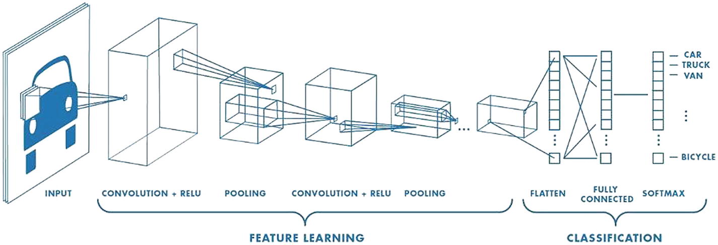
CNN is a special case of a neural network with an input layer, output layer, and multiple hidden layers. The hidden layers have 4 different procedures to complete the network. Each one is explained in detail.

Convolution
../images/475440_1_En_6_Chapter/475440_1_En_6_Figc_HTML.jpg

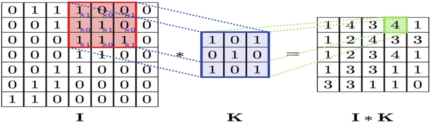
The Convolution layer is the heart of a Convolutional Neural Network, which does most of the computational operations. The name comes from the “convolution” operator that extracts features from the input image. These are also called filters (Orange color 3*3 matrix). The matrix formed by sliding the filter over the full image and calculating the dot product between these 2 matrices is called the ‘Convolved Feature’ or ‘Activation Map’ or the ‘Feature Map’. Suppose that in table data, different types of features are calculated like “age” from “date of birth.” The same way here also, straight edges, simple colors, and curves are some of the features that the filter will extract from the image.

During the training of the CNN, it learns the numbers or values present inside the filter and uses them on testing data. The greater the number of features, the more the image features get extracted and recognize all patterns in unseen images.

Nonlinearity (ReLU)
../images/475440_1_En_6_Chapter/475440_1_En_6_Figd_HTML.jpg

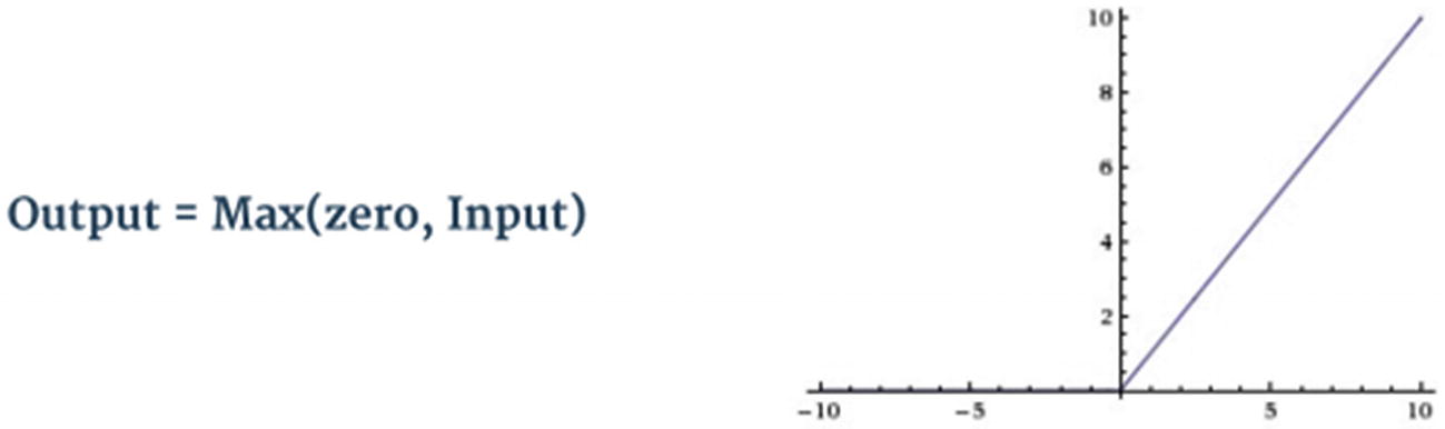
ReLU (Rectified Linear Unit) is a nonlinear function that is used after a convolution layer in CNN architecture. It replaces all negative values in the matrix to zero. The purpose of ReLU is to introduce nonlinearity in the CNN to perform better.

Pooling
../images/475440_1_En_6_Chapter/475440_1_En_6_Fige_HTML.jpg

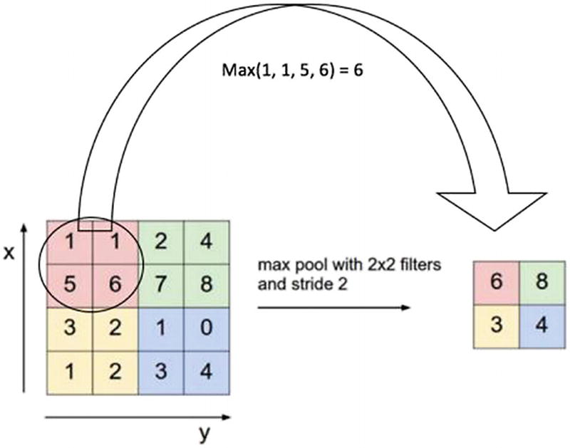
Pooling or subsampling is used to decrease the dimensionality of the feature without losing important information. It’s done to reduce the huge number of inputs to a full connected layer and computation required to process the model. It also helps to reduce the overfitting of the model. It uses a 2 x 2 window and slides over the image and takes the maximum value in each region as shown in the figure. This is how it reduces dimensionality.

Flatten, Fully Connected, and Softmax Layers

The last layer is a dense layer that needs feature vectors as input. But the output from the pooling layer is not a 1D feature vector. This process of converting the output of convolution to a feature vector is called flattening. The Fully Connected layer takes an input from the flatten layer and gives out an N-dimensional vector where N is the number of classes. The function of the fully connected layer is to use these features for classifying the input image into various classes based on the loss function on the training dataset. The Softmax function is used at the very end to convert these N-dimensional vectors into a probability for each class, which will eventually classify the image into a particular class.

Backpropagation: Training the Neural Network

In normal neural networks, you basically do Forward Propagation to get the output and check if this output is correct and calculate the error. In Backward Propagation, we are going backward through your network that finds the partial derivatives of the error with respect to each weight.

Let’s see how exactly it works.

The input image is fed into the network and completes forward propagation, which is convolution, ReLU, and pooling operations with forward propagation in the fully Connected layer and generates output probabilities for each class. As per the feed forward rule, weights are randomly assigned and complete the first iteration of training and also output random probabilities. After the end of the first step, the network calculates the error at the output layer using

Total Error = ∑ ½ (target probability – output probability) 2

Now, your backpropagation starts to calculate the gradients of the error with respect to all weights in the network and use gradient descent to update all filter values and weights, which will eventually minimize the output error. Parameters like the number of filters, filter sizes, and the architecture of the network will be finalized while building your network. The filter matrix and connection weights will get updated for each run. The whole process is repeated for the complete training set until the error is minimized.

Recurrent Neural Networks

CNNs are basically used for computer vision problems but fail to solve sequence models. Sequence models are those where even a sequence of the entity also matters. For example, in the text, the order of the words matters to create meaningful sentences. This is where RNNs come into the picture and are useful with sequential data because each neuron can use its memory to remember information about the previous step.

../images/475440_1_En_6_Chapter/475440_1_En_6_Figf_HTML.jpg

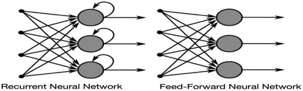
It is quite complex to understand how exactly RNN is working. If you see the above figure, the recurrent neural network is taking the output from the hidden layer and sending it back to the same layer before giving the prediction.

Training RNN – Backpropagation Through Time (BPTT)

We know how feed forward and backpropagation work from CNN, so let’s see how training is done in case of RNN.

../images/475440_1_En_6_Chapter/475440_1_En_6_Figg_HTML.jpg

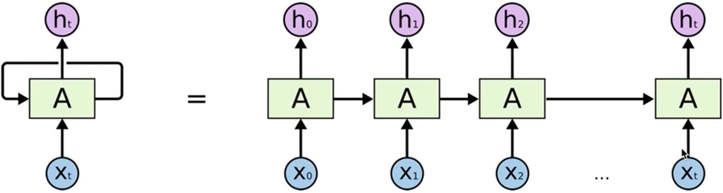
If we just discuss the hidden layer, it’s not only taking input from the hidden layer, but we can also add another input to the same hidden layer. Now the backpropagation happens like any other previous training we have seen; it’s just that now it is dependent on time. Here error is backpropagated from the last timestamp to the first through unrolling the hidden layers. This allows calculating the error for each timestamp and updating the weights. Recurrent networks with recurrent connections between hidden units read an entire sequence and then produce a required output.

When the values of a gradient are too small and the model takes way too long to learn, this is called Vanishing Gradients. This problem is solved by LSTMs.

Long Short-Term Memory (LSTM)

LSTMs are a kind of RNNs with betterment in equation and backpropagation, which makes it perform better. LSTMs work almost similarly to RNN, but these units can learn things with very long time gaps, and they can store information just like computers.

../images/475440_1_En_6_Chapter/475440_1_En_6_Figh_HTML.jpg

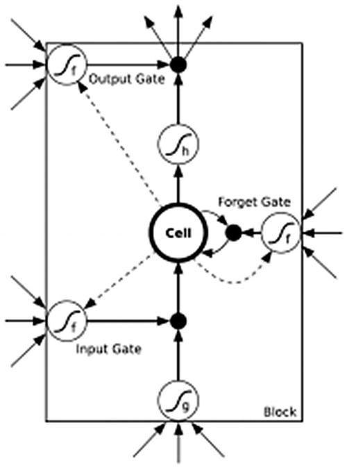
The algorithm learns the importance of the word or character through weighing methodology and decides whether to store it or not. For this, it uses regulated structures called gates that have the ability to remove or add information to the cell. These cells have a sigmoid layer that decides how much information should be passed. It has three layers, namely “input,” “forget,” and “output” to carry out this process.

Going in depth on how CNN and RNNs work is beyond the scope of this book. We have mentioned references at the end of the book if anyone is interested in learning about this in more depth.

Recipe 6-1. Retrieving Information

Information retrieval is one of the highly used applications of NLP and it is quite tricky. The meaning of the words or sentences not only depends on the exact words used but also on the context and meaning. Two sentences may be of completely different words but can convey the same meaning. We should be able to capture that as well.

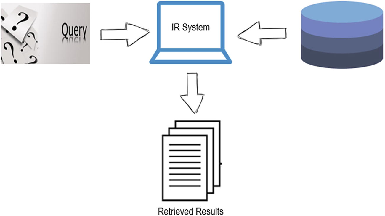
An information retrieval (IR) system allows users to efficiently search documents and retrieve meaningful information based on a search text/query.

../images/475440_1_En_6_Chapter/475440_1_En_6_Figi_HTML.jpg

Problem

Information retrieval using word embeddings.

Solution

There are multiple ways to do Information retrieval. But we will see how to do it using word embeddings, which is very effective since it takes context also into consideration. We discussed how word embeddings are built in Chapter 3. We will just use the pretrained word2vec in this case.

Let’s take a simple example and see how to build a document retrieval using query input. Let’s say we have 4 documents in our database as below. (Just showcasing how it works. We will have too many documents in a real-world application.)
Doc1 = ["With the Union cabinet approving the amendments to the Motor Vehicles Act, 2016, those caught for drunken driving will have to have really deep pockets, as the fine payable in court has been enhanced to Rs 10,000 for first-time offenders." ]
Doc2 = ["Natural language processing (NLP) is an area of computer science and artificial intelligence concerned with the interactions between computers and human (natural) languages, in particular how to program computers to process and analyze large amounts of natural language data."]
Doc3 = ["He points out that public transport is very good in Mumbai and New Delhi, where there is a good network of suburban and metro rail systems."]
Doc4 = ["But the man behind the wickets at the other end was watching just as keenly. With an affirmative nod from Dhoni, India captain Rohit Sharma promptly asked for a review. Sure enough, the ball would have clipped the top of middle and leg."]
Assume we have numerous documents like this. And you want to retrieve the most relevant once for the query “cricket.” Let’s see how to build it.
query = "cricket"

How It Works

Step 1-1 Import the libraries

Here are the libraries:
import gensim
from gensim.models import Word2Vec
import numpy as np
import nltk
import itertools
from nltk.corpus import stopwords
from nltk.tokenize import sent_tokenize, word_tokenize
import scipy
from scipy import spatial
from nltk.tokenize.toktok import ToktokTokenizer
import re
tokenizer = ToktokTokenizer()
stopword_list = nltk.corpus.stopwords.words('english')   

Step 1-2 Create/import documents

Randomly taking sentences from the internet:
Doc1 = ["With the Union cabinet approving the amendments to the Motor Vehicles Act, 2016, those caught for drunken driving will have to have really deep pockets, as the fine payable in court has been enhanced to Rs 10,000 for first-time offenders." ]
Doc2 = ["Natural language processing (NLP) is an area of computer science and artificial intelligence concerned with the interactions between computers and human (natural) languages, in particular how to program computers to process and analyze large amounts of natural language data."]
Doc3 = ["He points out that public transport is very good in Mumbai and New Delhi, where there is a good network of suburban and metro rail systems."]
Doc4 = ["But the man behind the wickets at the other end was watching just as keenly. With an affirmative nod from Dhoni, India captain Rohit Sharma promptly asked for a review. Sure enough, the ball would have clipped the top of middle and leg."]
# Put all the documents in one list
fin= Doc1+Doc2+Doc3+Doc4

Step 1-3 Download word2vec

As mentioned earlier, we are going to use the word embeddings to solve this problem. Download word2vec from the below link:
https://drive.google.com/file/d/0B7XkCwpI5KDYNlNUTTlSS21pQmM/edit
#load the model
model = gensim.models.KeyedVectors.load_word2vec_format('/GoogleNews-vectors-negative300.bin', binary=True)

Step 1-4 Create IR system

Now we build the information retrieval system:
#Preprocessing
def remove_stopwords(text, is_lower_case=False):
    pattern = r'[^a-zA-z0-9s]'
    text = re.sub(pattern, ", ".join(text))
    tokens = tokenizer.tokenize(text)
    tokens = [token.strip() for token in tokens]
    if is_lower_case:
        filtered_tokens = [token for token in tokens if token not in stopword_list]
    else:
        filtered_tokens = [token for token in tokens if token.lower() not in stopword_list]
    filtered_text = ' '.join(filtered_tokens)
    return filtered_text
# Function to get the embedding vector for n dimension, we have used "300"
def get_embedding(word):
    if word in model.wv.vocab:
        return model[x]
    else:
        return np.zeros(300)
For every document, we will get a lot of vectors based on the number of words present. We need to calculate the average vector for the document through taking a mean of all the word vectors.
# Getting average vector for each document
out_dict =  {}
for sen in fin:
    average_vector = (np.mean(np.array([get_embedding(x) for x in nltk.word_tokenize(remove_stopwords(sen))]), axis=0))
    dict = { sen : (average_vector) }
    out_dict.update(dict)
# Function to calculate the similarity between the query vector and document vector
def get_sim(query_embedding, average_vector_doc):
    sim = [(1 - scipy.spatial.distance.cosine(query_embedding, average_vector_doc))]
    return sim
# Rank all the documents based on the similarity to get relevant docs
def Ranked_documents(query):
    query_words =  (np.mean(np.array([get_embedding(x) for x in nltk.word_tokenize(query.lower())],dtype=float), axis=0))
    rank = []
    for k,v in out_dict.items():
        rank.append((k, get_sim(query_words, v)))
    rank = sorted(rank,key=lambda t: t[1], reverse=True)
    print('Ranked Documents :')
    return rank

Step 1-5 Results and applications

Let’s see how the information retrieval system we built is working with a couple of examples.
# Call the IR function with a query
Ranked_documents("cricket")
Result :
[('But the man behind the wickets at the other end was watching just as keenly. With an affirmative nod from Dhoni, India captain Rohit Sharma promptly asked for a review. Sure enough, the ball would have clipped the top of middle and leg.',
  [0.44954327116871795]),
 ('He points out that public transport is very good in Mumbai and New Delhi, where there is a good network of suburban and metro rail systems.',
  [0.23973446569030055]),
 ('With the Union cabinet approving the amendments to the Motor Vehicles Act, 2016, those caught for drunken driving will have to have really deep pockets, as the fine payable in court has been enhanced to Rs 10,000 for first-time offenders.',
  [0.18323712012013349]),
 ('Natural language processing (NLP) is an area of computer science and artificial intelligence concerned with the interactions between computers and human (natural) languages, in particular how to program computers to process and analyze large amounts of natural language data.',
  [0.17995060855459855])]

If you see, doc4 (on top in result), this will be most relevant for the query “cricket” even though the word “cricket” is not even mentioned once with the similarity of 0.449.

Let’s take one more example as may be driving.
Ranked_documents("driving")
[('With the Union cabinet approving the amendments to the Motor Vehicles Act, 2016, those caught for drunken driving will have to have really deep pockets, as the fine payable in court has been enhanced to Rs 10,000 for first-time offenders.',
  [0.35947287723800669]),
 ('But the man behind the wickets at the other end was watching just as keenly. With an affirmative nod from Dhoni, India captain Rohit Sharma promptly asked for a review. Sure enough, the ball would have clipped the top of middle and leg.',
  [0.19042556935316801]),
 ('He points out that public transport is very good in Mumbai and New Delhi, where there is a good network of suburban and metro rail systems.',
  [0.17066536985237601]),
 ('Natural language processing (NLP) is an area of computer science and artificial intelligence concerned with the interactions between computers and human (natural) languages, in particular how to program computers to process and analyze large amounts of natural language data.',
  [0.088723080005327359])]

Again, since driving is connected to transport and the Motor Vehicles Act, it pulls out the most relevant documents on top. The first 2 documents are relevant to the query.

We can use the same approach and scale it up for as many documents as possible. For more accuracy, we can build our own embeddings, as we learned in Chapter 3, for specific industries since the one we are using is generalized.

This is the fundamental approach that can be used for many applications like the following:
  • Search engines

  • Document retrieval

  • Passage retrieval

  • Question and answer

../images/475440_1_En_6_Chapter/475440_1_En_6_Figj_HTML.jpg

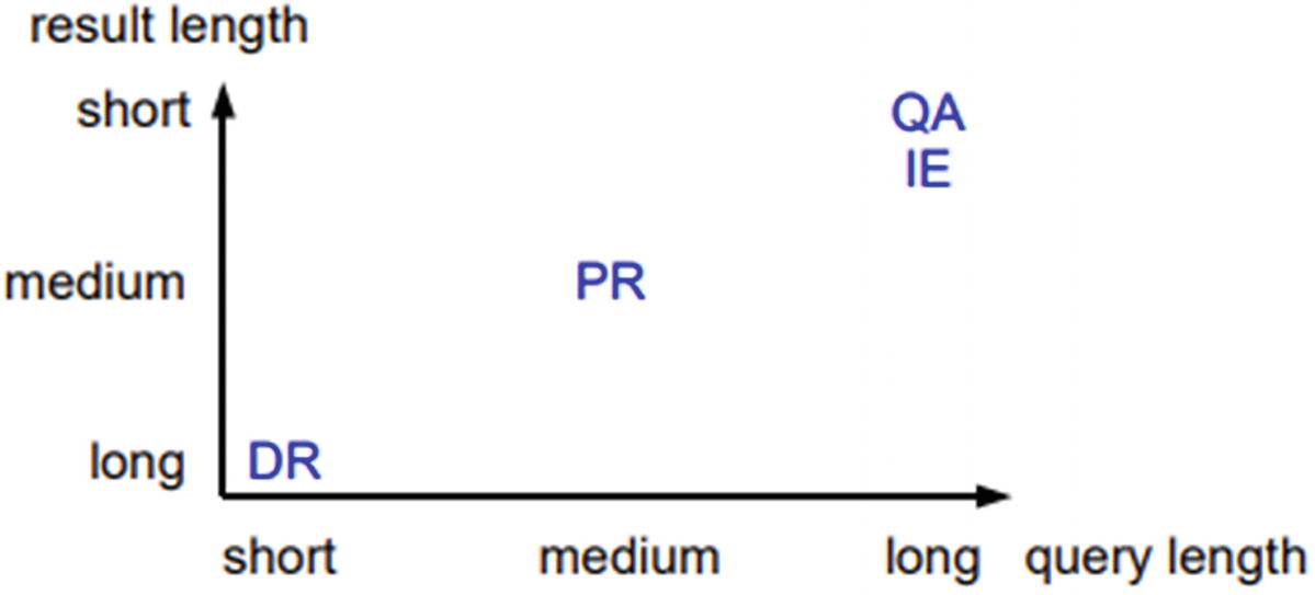
It’s been proven that results will be good when queries are longer and the result length is shorter. That’s the reason we don’t get great results in search engines when the search query has lesser number of words.

Recipe 6-2. Classifying Text with Deep Learning

In this recipe, let us build a text classifier using deep learning approaches.

Problem

We want to build a text classification model using CNN, RNN, and LSTM.

Solution

The approach and NLP pipeline would remain the same as discussed earlier. The only change would be that instead of using machine learning algorithms, we would be building models using deep learning algorithms.

How It Works

Let’s follow the steps in this section to build the email classifier using the deep learning approaches.

Step 2-1 Understanding/defining business problem

Email classification (spam or ham) . We need to classify spam or ham email based on email content.

Step 2-2 Identifying potential data sources, collection, and understanding

Using the same data used in Recipe 4-6 from Chapter 4:
#read file
file_content = pd.read_csv('spam.csv', encoding = "ISO-8859-1")
#check sample content in the email
file_content['v2'][1]
#output
'Ok lar... Joking wif u oni...'

Step 2-3 Text preprocessing

Let’s preprocess the data:
#Import library
from nltk.corpus import stopwords
from nltk import *
from sklearn.feature_extraction.text import TfidfVectorizer
from nltk.stem import WordNetLemmatizer
import matplotlib.pyplot as plt
from sklearn.model_selection import train_test_split
# Remove stop words
stop = stopwords.words('english')
file_content['v2'] = file_content['v2'].apply(lambda x: " ".join(x for x in x.split() if x not in stop))
# Delete unwanted columns
Email_Data = file_content[['v1', 'v2']]
# Rename column names
Email_Data = Email_Data.rename(columns={"v1":"Target", "v2":"Email"})
Email_Data.head()
 #output
    Target Email
0   ham    Go jurong point, crazy.. Available bugis n gre...
1   ham    Ok lar... Joking wif u oni...
2   spam   Free entry 2 wkly comp win FA Cup final tkts 2...
3   ham    U dun say early hor... U c already say...
4   ham    Nah I think goes usf, lives around though
#Delete punctuations, convert text in lower case and delete the double space
Email_Data['Email'] = Email_Data['Email'].apply(lambda x: re.sub('[!@#$:).;,?&]', ", x.lower()))
Email_Data['Email'] = Email_Data['Email'].apply(lambda x: re.sub(' ', ' ', x))
Email_Data['Email'].head(5)
#output
0 go jurong point crazy available bugis n great ...
1 ok lar joking wif u oni
2 free entry 2 wkly comp win fa cup final tkts 2...
3 u dun say early hor u c already say
4 nah i think goes usf lives around though
Name: Email, dtype: object
#Separating text(input) and target classes
list_sentences_rawdata = Email_Data["Email"].fillna("_na_").values
list_classes = ["Target"]
target = Email_Data[list_classes].values
To_Process=Email_Data[['Email', 'Target']]

Step 2-4 Data preparation for model building

Now we prepare the data:
#Train and test split with 80:20 ratio
train, test = train_test_split(To_Process, test_size=0.2)
# Define the sequence lengths, max number of words and embedding dimensions
# Sequence length of each sentence. If more, truncate. If less, pad with zeros
MAX_SEQUENCE_LENGTH = 300
# Top 20000 frequently occurring words
MAX_NB_WORDS = 20000
# Get the frequently occurring words
 tokenizer = Tokenizer(num_words=MAX_NB_WORDS)
tokenizer.fit_on_texts(train.Email)
train_sequences = tokenizer.texts_to_sequences(train.Email)
test_sequences = tokenizer.texts_to_sequences(test.Email)
# dictionary containing words and their index
word_index = tokenizer.word_index
# print(tokenizer.word_index)
# total words in the corpus
print('Found %s unique tokens.' % len(word_index))
# get only the top frequent words on train
train_data = pad_sequences(train_sequences, maxlen=MAX_SEQUENCE_LENGTH)
# get only the top frequent words on test
test_data = pad_sequences(test_sequences, maxlen=MAX_SEQUENCE_LENGTH)
print(train_data.shape)
print(test_data.shape)
#output
Found 8443 unique tokens.
(4457, 300)
(1115, 300)
train_labels = train['Target']
test_labels = test['Target']
#import library
from sklearn.preprocessing import LabelEncoder
# converts the character array to numeric array. Assigns levels to unique labels.
le = LabelEncoder()
le.fit(train_labels)
train_labels = le.transform(train_labels)
test_labels = le.transform(test_labels)
print(le.classes_)
print(np.unique(train_labels, return_counts=True))
print(np.unique(test_labels, return_counts=True))
#output
['ham' 'spam']
(array([0, 1]), array([3889, 568]))
(array([0, 1]), array([936, 179]))
# changing data types
labels_train = to_categorical(np.asarray(train_labels))
labels_test = to_categorical(np.asarray(test_labels))
print('Shape of data tensor:', train_data.shape)
print('Shape of label tensor:', labels_train.shape)
print('Shape of label tensor:', labels_test.shape)
#output
Shape of data tensor: (4457, 300)
Shape of label tensor: (4457, 2)
Shape of label tensor: (1115, 2)
EMBEDDING_DIM = 100
print(MAX_SEQUENCE_LENGTH)
#output
300

Step 2-5 Model building and predicting

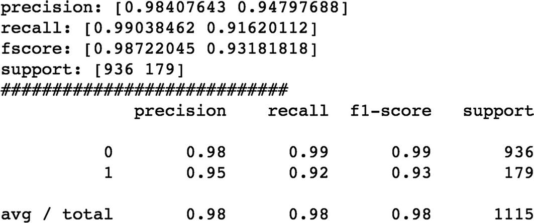
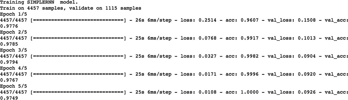
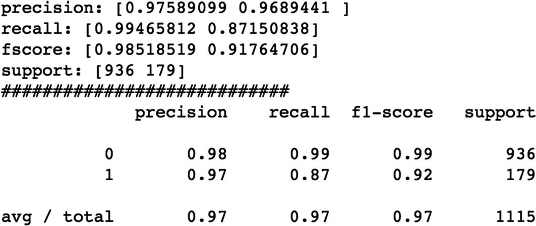
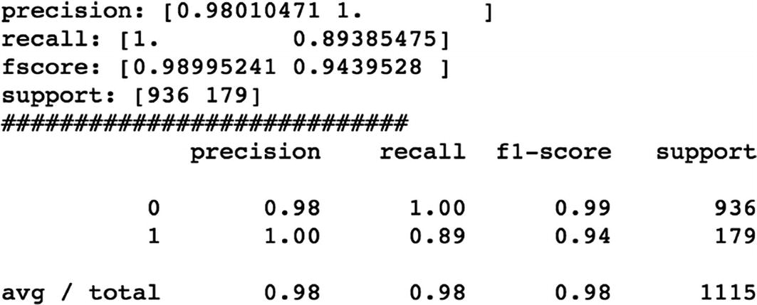
We are building the models using different deep learning approaches like CNN, RNN, LSTM, and Bidirectional LSTM and comparing the performance of each model using different accuracy metrics.

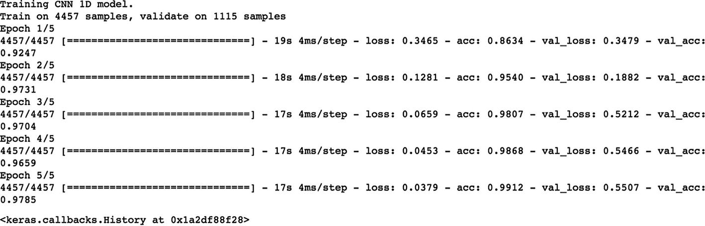
We can now define our CNN model.

Here we define a single hidden layer with 128 memory units. The network uses a dropout with a probability of 0.5. The output layer is a dense layer using the softmax activation function to output a probability prediction.
# Import Libraries
import sys, os, re, csv, codecs, numpy as np, pandas as pd
from keras.preprocessing.text import Tokenizer
from keras.preprocessing.sequence import pad_sequences
from keras.utils import to_categorical
from keras.layers import Dense, Input, LSTM, Embedding, Dropout, Activation
from keras.layers import Bidirectional, GlobalMaxPool1D, Conv1D, SimpleRNN
from keras.models import Model
from keras.models import Sequential
from keras import initializers, regularizers, constraints, optimizers, layers
from keras.layers import Dense, Input, Flatten, Dropout, BatchNormalization
from keras.layers import Conv1D, MaxPooling1D, Embedding
from keras.models import Sequential
 print('Training CNN 1D model.')
model = Sequential()
model.add(Embedding(MAX_NB_WORDS,
 EMBEDDING_DIM,
 input_length=MAX_SEQUENCE_LENGTH
 ))
model.add(Dropout(0.5))
model.add(Conv1D(128, 5, activation="relu"))
model.add(MaxPooling1D(5))
model.add(Dropout(0.5))
model.add(BatchNormalization())
model.add(Conv1D(128, 5, activation="relu"))
model.add(MaxPooling1D(5))
model.add(Dropout(0.5))
model.add(BatchNormalization())
model.add(Flatten())
model.add(Dense(128, activation="relu"))
model.add(Dense(2, activation="softmax"))
model.compile(loss='categorical_crossentropy',
 optimizer="rmsprop",
 metrics=['acc'])
We are now fitting our model to the data. Here we have 5 epochs and a batch size of 64 patterns.
model.fit(train_data, labels_train,
 batch_size=64,
 epochs=5,
 validation_data=(test_data, labels_test))
#output
../images/475440_1_En_6_Chapter/475440_1_En_6_Figk_HTML.jpg
#predictions on test data
predicted=model.predict(test_data)
predicted
#output
array([[0.5426713 , 0.45732868],
 [0.5431667 , 0.45683333],
 [0.53082496, 0.46917507],
 ...,
 [0.53582424, 0.46417573],
 [0.5305845 , 0.46941552],
 [0.53102577, 0.46897423]], dtype=float32)
#model evaluation
import sklearn
from sklearn.metrics import precision_recall_fscore_support as score
precision, recall, fscore, support = score(labels_test, predicted.round())
print('precision: {}'.format(precision))
print('recall: {}'.format(recall))
print('fscore: {}'.format(fscore))
print('support: {}'.format(support))
print("############################")
print(sklearn.metrics.classification_report(labels_test, predicted.round()))
#output
../images/475440_1_En_6_Chapter/475440_1_En_6_Figl_HTML.jpg
We can now define our RNN model.
#import library
from keras.layers.recurrent import SimpleRNN
#model training
print('Training SIMPLERNN model.')
model = Sequential()
model.add(Embedding(MAX_NB_WORDS,
 EMBEDDING_DIM,
 input_length=MAX_SEQUENCE_LENGTH
 ))
model.add(SimpleRNN(2, input_shape=(None,1)))
model.add(Dense(2,activation='softmax'))
model.compile(loss = 'binary_crossentropy', optimizer="adam",metrics = ['accuracy'])
model.fit(train_data, labels_train,
 batch_size=16,
 epochs=5,
 validation_data=(test_data, labels_test))
#output
../images/475440_1_En_6_Chapter/475440_1_En_6_Figm_HTML.jpg
# prediction on test data
predicted_Srnn=model.predict(test_data)
predicted_Srnn
#output
array([[0.9959137 , 0.00408628],
 [0.99576926, 0.00423072],
 [0.99044365, 0.00955638],
 ...,
 [0.9920791 , 0.00792089],
 [0.9958105 , 0.00418955],
 [0.99660563, 0.00339443]], dtype=float32)
#model evaluation
from sklearn.metrics import precision_recall_fscore_support as score
precision, recall, fscore, support = score(labels_test, predicted_Srnn.round())
print('precision: {}'.format(precision))
print('recall: {}'.format(recall))
print('fscore: {}'.format(fscore))
print('support: {}'.format(support))
print("############################")
print(sklearn.metrics.classification_report(labels_test, predicted_Srnn.round()))
#output
../images/475440_1_En_6_Chapter/475440_1_En_6_Fign_HTML.jpg
And here is our Long Short-Term Memory (LSTM):
#model training
print('Training LSTM model.')
model = Sequential()
model.add(Embedding(MAX_NB_WORDS,
 EMBEDDING_DIM,
 input_length=MAX_SEQUENCE_LENGTH
 ))
model.add(LSTM(output_dim=16, activation="relu", inner_activation="hard_sigmoid",return_sequences=True))
model.add(Dropout(0.2))
model.add(BatchNormalization())
model.add(Flatten())
model.add(Dense(2,activation='softmax'))
model.compile(loss = 'binary_crossentropy', optimizer="adam",metrics = ['accuracy'])
model.fit(train_data, labels_train,
 batch_size=16,
 epochs=5,
 validation_data=(test_data, labels_test))
#output
../images/475440_1_En_6_Chapter/475440_1_En_6_Figo_HTML.jpg
#prediction on text data
predicted_lstm=model.predict(test_data)
predicted_lstm
array([[1.0000000e+00, 4.0581045e-09],
 [1.0000000e+00, 8.3188789e-13],
 [9.9999976e-01, 1.8647323e-07],
 ...,
 [9.9999976e-01, 1.8333606e-07],
 [1.0000000e+00, 1.7347950e-09],
 [9.9999988e-01, 1.3574694e-07]], dtype=float32)
#model evaluation
from sklearn.metrics import precision_recall_fscore_support as score
precision, recall, fscore, support = score(labels_test, predicted_lstm.round())
print('precision: {}'.format(precision))
print('recall: {}'.format(recall))
print('fscore: {}'.format(fscore))
print('support: {}'.format(support))
print("############################")
print(sklearn.metrics.classification_report(labels_test, predicted_lstm.round()))
#output
../images/475440_1_En_6_Chapter/475440_1_En_6_Figp_HTML.jpg

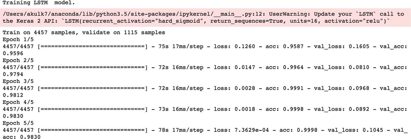
Finally, let’s see what is Bidirectional LSTM and implement the same.

As we know, LSTM preserves information from inputs using the hidden state. In bidirectional LSTMs, inputs are fed in two ways: one from previous to future and the other going backward from future to past, helping in learning future representation as well. Bidirectional LSTMs are known for producing very good results as they are capable of understanding the context better.
#model training
print('Training Bidirectional LSTM model.')
model = Sequential()
model.add(Embedding(MAX_NB_WORDS,
 EMBEDDING_DIM,
 input_length=MAX_SEQUENCE_LENGTH
 ))
model.add(Bidirectional(LSTM(16, return_sequences=True, dropout=0.1, recurrent_dropout=0.1)))
model.add(Conv1D(16, kernel_size = 3, padding = "valid", kernel_initializer = "glorot_uniform"))
model.add(GlobalMaxPool1D())
model.add(Dense(50, activation="relu"))
model.add(Dropout(0.1))
model.add(Dense(2,activation='softmax'))
model.compile(loss = 'binary_crossentropy', optimizer="adam",metrics = ['accuracy'])
model.fit(train_data, labels_train,
 batch_size=16,
 epochs=3,
 validation_data=(test_data, labels_test))
#output
../images/475440_1_En_6_Chapter/475440_1_En_6_Figq_HTML.jpg
# prediction on test data
predicted_blstm=model.predict(test_data)
predicted_blstm
#output
array([[9.9999976e-01, 2.6086647e-07],
 [9.9999809e-01, 1.9633851e-06],
 [9.9999833e-01, 1.6918856e-06],
 ...,
 [9.9999273e-01, 7.2622524e-06],
 [9.9999964e-01, 3.3541210e-07],
 [9.9999964e-01, 3.5427794e-07]], dtype=float32)
#model evaluation
from sklearn.metrics import precision_recall_fscore_support as score
precision, recall, fscore, support = score(labels_test, predicted_blstm.round())
print('precision: {}'.format(precision))
print('recall: {}'.format(recall))
print('fscore: {}'.format(fscore))
print('support: {}'.format(support))
print("############################")
print(sklearn.metrics.classification_report(labels_test, predicted_blstm.round()))
#output
../images/475440_1_En_6_Chapter/475440_1_En_6_Figr_HTML.jpg

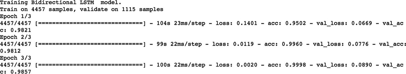
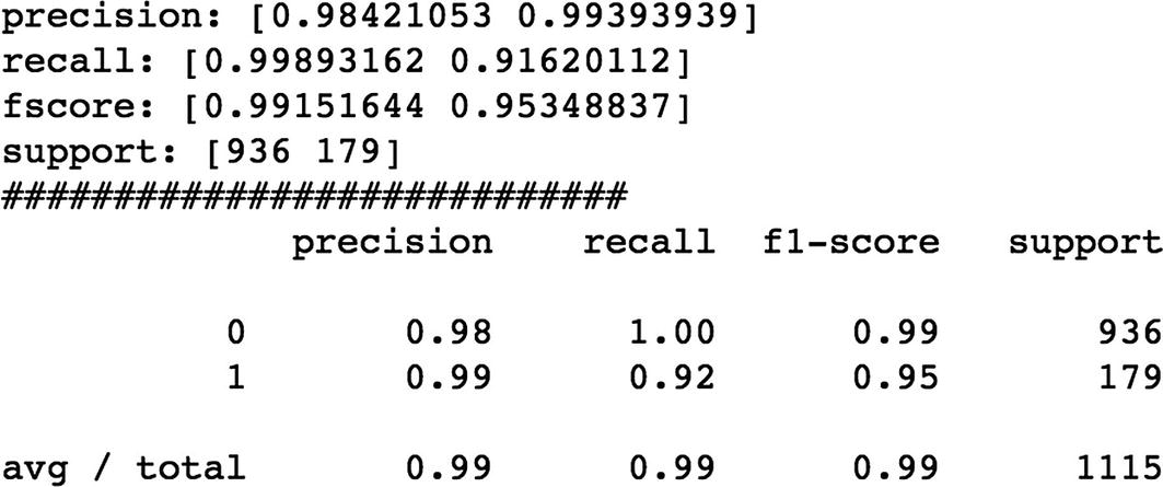
We can see that Bidirectional LSTM outperforms the rest of the algorithms.

Recipe 6-3. Next Word Prediction

Autofill/showing what could be the potential sequence of words saves a lot of time while writing emails and makes users happy to use it in any product.

Problem

You want to build a model to predict/suggest the next word based on a previous sequence of words using Email Data.

Like you see in the below image, language is being suggested as the next word.

../images/475440_1_En_6_Chapter/475440_1_En_6_Figs_HTML.jpg

Solution

In this section, we will build an LSTM model to learn sequences of words from email data. We will use this model to predict the next word.

How It Works

Let's follow the steps in this section to build the next word prediction model using the deep learning approach.

Step 3-1 Understanding/defining business problem

Predict the next word based on the sequence of words or sentences.

Step 3-2 Identifying potential data sources, collection, and understanding

For this problem, let us use the same email data used in Recipe 4-6 from Chapter 4. This has a lot less data, but still to showcase the working flow, we are fine with this data. The more data, the better the accuracy.
file_content = pd.read_csv('spam.csv', encoding = "ISO-8859-1")
# Just selecting emails and connverting it into list
Email_Data = file_content[[ 'v2']]
list_data = Email_Data.values.tolist()
list_data
#output
[['Go until jurong point, crazy.. Available only in bugis n great world la e buffet... Cine there got amore wat...'],
 ['Ok lar... Joking wif u oni...'],
 ["Free entry in 2 a wkly comp to win FA Cup final tkts 21st May 2005. Text FA to 87121 to receive entry question(std txt rate)T&C's apply 08452810075over18's"],
 ['U dun say so early hor... U c already then say...'],
 ["Nah I don't think he goes to usf, he lives around here though"],
 ["FreeMsg Hey there darling it's been 3 week's now and no word back! I'd like some fun you up for it still? Tb ok! XxX std chgs to send, å£1.50 to rcv"],
 ['Even my brother is not like to speak with me. They treat me like aids patent.'],
 ["As per your request 'Melle Melle (Oru Minnaminunginte Nurungu Vettam)' has been set as your callertune for all Callers. Press *9 to copy your friends Callertune"],
 ['WINNER!! As a valued network customer you have been selected to receivea å£900 prize reward! To claim call 09061701461. Claim code KL341. Valid 12 hours only.'] ,
 ['Had your mobile 11 months or more? U R entitled to Update to the latest colour mobiles with camera for Free! Call The Mobile Update Co FREE on 08002986030'],

Step 3-3 Importing and installing necessary libraries

Here are the libraries:
import numpy as np
import random
import pandas as pd
import sys
import os
import time
import codecs
import collections
import numpy
from keras.models import Sequential
from keras.layers import Dense
from keras.layers import Dropout
from keras.layers import LSTM
from keras.callbacks import ModelCheckpoint
from keras.utils import np_utils
from nltk.tokenize import sent_tokenize, word_tokenize
import scipy
from scipy import spatial
from nltk.tokenize.toktok import ToktokTokenizer
import re
tokenizer = ToktokTokenizer()

Step 3-4 Processing the data

Now we process the data:
#Converting list to string
from collections import Iterable
def flatten(items):
    """Yield items from any nested iterable"""
    for x in items:
        if isinstance(x, Iterable) and not isinstance(x, (str, bytes)):
            for sub_x in flatten(x):
                yield sub_x
        else:
            yield x
TextData=list(flatten(list_data))
TextData = ".join(TextData)
# Remove unwanted lines and converting into lower case
TextData = TextData.replace(' ',")
TextData = TextData.lower()
pattern = r'[^a-zA-z0-9s]'
TextData = re.sub(pattern, ", ".join(TextData))
# Tokenizing
tokens = tokenizer.tokenize(TextData)
tokens = [token.strip() for token in tokens]
# get the distinct words and sort it
word_counts = collections.Counter(tokens)
word_c = len(word_counts)
print(word_c)
distinct_words = [x[0] for x in word_counts.most_common()]
distinct_words_sorted = list(sorted(distinct_words))
# Generate indexing for all words
word_index = {x: i for i, x in enumerate(distinct_words_sorted)}
# decide on sentence length
sentence_length = 25

Step 3-5 Data preparation for modeling

Here we are dividing the mails into sequence of words with a fixed length of 10 words (you can choose anything based on the business problem and computation power). We are splitting the text by words sequences. When creating these sequences, we slide this window along the whole document one word at a time, allowing each word to learn from its preceding one.
#prepare the dataset of input to output pairs encoded as integers
# Generate the data for the model
#input = the input sentence to the model with index
#output = output of the model with index
InputData = []
OutputData = []
for i in range(0, word_c - sentence_length, 1):
    X = tokens[i:i + sentence_length]
    Y = tokens[i + sentence_length]
    InputData.append([word_index[char] for char in X])
    OutputData.append(word_index[Y])
print (InputData[:1])
print (" ")
print(OutputData[:1])
#output
[[5086, 12190, 6352, 9096, 3352, 1920, 8507, 5937, 2535, 7886, 5214, 12910, 6541, 4104, 2531, 2997, 11473, 5170, 1595, 12552, 6590, 6316, 12758, 12087, 8496]]
[4292]
# Generate  X
X = numpy.reshape(InputData, (len(InputData), sentence_length, 1))
# One hot encode the output variable
Y = np_utils.to_categorical(OutputData)
Y
#output
array([[0., 0., 0., ..., 0., 0., 0.],
       [0., 0., 0., ..., 0., 0., 0.],
       [0., 0., 0., ..., 0., 0., 0.],
       ...,
       [0., 0., 0., ..., 0., 0., 0.],
       [0., 0., 0., ..., 0., 0., 0.],
       [0., 0., 0., ..., 0., 0., 0.]])

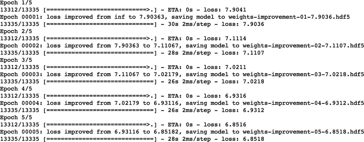
Step 3-6 Model building

We will now define the LSTM model. Here we define a single hidden LSTM layer with 256 memory units. This model uses dropout 0.2. The output layer is using the softmax activation function. Here we are using the ADAM optimizer.
# define the LSTM model
model = Sequential()
model.add(LSTM(256, input_shape=(X.shape[1], X.shape[2])))
model.add(Dropout(0.2))
model.add(Dense(Y.shape[1], activation="softmax"))
model.compile(loss='categorical_crossentropy', optimizer="adam")
#define the checkpoint
file_name_path="weights-improvement-{epoch:02d}-{loss:.4f}.hdf5"
checkpoint = ModelCheckpoint(file_name_path, monitor="loss", verbose=1, save_best_only=True, mode="min")
callbacks = [checkpoint]
We can now fit the model to the data. Here we use 5 epochs and a batch size of 128 patterns. For better results, you can use more epochs like 50 or 100. And of course, you can use them on more data.
#fit the model
model.fit(X, Y, epochs=5, batch_size=128, callbacks=callbacks)

Note

We have not split the data into training and testing data. We are not interested in the accurate model. As we all know, deep learning models will require a lot of data for training and take a lot of time to train, so we are using a model checkpoint to capture all of the model weights to file. We will use the best set of weights for our prediction.

#output
../images/475440_1_En_6_Chapter/475440_1_En_6_Figt_HTML.jpg
After running the above code, you will have weight checkpoint files in your local directory. Pick the network weights file that is saved in your working directory. For example, when we ran this example, below was the checkpoint with the smallest loss that we achieved with 5 epochs.
# load the network weights
file_name = "weights-improvement-05-6.8213.hdf5"
model.load_weights(file_name)
model.compile(loss='categorical_crossentropy', optimizer="adam")

Step 3-7 Predicting next word

We will randomly generate a sequence of words and input to the model and see what it predicts.
# Generating random sequence
start = numpy.random.randint(0, len(InputData))
input_sent = InputData[start]
# Generate index of the next word of the email
X = numpy.reshape(input_sent, (1, len(input_sent), 1))
predict_word = model.predict(X, verbose=0)
index = numpy.argmax(predict_word)
print(input_sent)
print (" ")
print(index)
# Output
[9122, 1920, 8187, 5905, 6828, 9818, 1791, 5567, 1597, 7092, 11606, 7466, 10198, 6105, 1837, 4752, 7092, 3928, 10347, 5849, 8816, 7092, 8574, 7092, 1831]
5849
# Convert these indexes back to words
word_index_rev = dict((i, c) for i, c in enumerate(tokens))
result = word_index_rev[index]
sent_in = [word_index_rev[value] for value in input_sent]
print(sent_in)
print (" ")
print(result)
Result :
['us', 'came', 'use', 'respecthe', 'would', 'us', 'are', 'it', 'you', 'to', 'pray', 'because', 'you', 'do', 'me', 'out', 'youre', 'thk', 'where', 'are', 'mrng', 'minutes', 'long', '500', 'per']
shut

So, given the 25 input words, it's predicting the word “shut” as the next word. Of course, its not making much sense, since it has been trained on much less data and epochs. Make sure you have great computation power and train on huge data with high number of epochs.

..................Content has been hidden....................

You can't read the all page of ebook, please click here login for view all page.
Reset
18.117.142.230