© Alejandro Serrano Mena 2019
Alejandro Serrano MenaPractical Haskellhttps://doi.org/10.1007/978-1-4842-4480-7_3

3. Increasing Code Reuse

Alejandro Serrano Mena1 
(1)
Utrecht, The Netherlands
 

Chapter 1 explained that a functional language like Haskell is characterized by its profuse use of functions as parameters or return values. However, Chapter 2 didn’t mention anything about this topic. I’ll rectify that here. In this chapter, you will focus on not one but three ways in which Haskell allows for a great amount of reuse.

One of the ways in which Haskell shines in the area of reusability is through the creation of functions that can work over values of any type that respects a certain form, or design. List functions such as head can operate on any type of the form [T], whatever type T is. This concept is also applicable to data types that can store values on any possible type, which is known as parametric polymorphism .

Another way in which Haskell allows for reuse is this ability of using functions as any other value of the language. Functions that manipulate other functions are called higher-order functions. In contrast, the concepts in the previous chapter belong to first-order Haskell.

The third way in which code can be reused (and shared) is by taking functions or data types from one module and applying them in another. You will learn how to do that from both sides: exporting definitions to make them available and importing them later.

Most of the examples in this chapter focus on lists and the functions in the module Data.List. The intention is twofold: lists illustrate the new concepts to be introduced, and at the same time they are practical tools in daily programming with Haskell. As proof of their importance, the language includes special syntax to create and manage them, namely, the syntax of comprehensions. I’ll explain how to use the syntax before moving to the last stop of the list train: how to fold and unfold lists properly.

Parametric Polymorphism

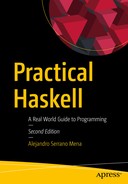
You may have noticed that in previous chapters all the functions defined operated on some particular data type. However, some built-in functions such as head or empty seem to be able to operate on any kind of list: [Integer], [Client], and so forth. A fair question is, are list functions somehow treated differently by the compiler and interpreter, or do I also have the power to create such functions that can operate on any type? The correct answer is the latter: you could have defined the list functions by yourself with no problem. You do have the power.

Let’s look at the type of a function such as head:
*Chapter3.ParamPoly> :t head
head :: [a] -> a

In the previous chapter you learned that type names must start with an uppercase letter. However, you can see a lowercase identifier in this particular signature. If you remember the conventions, you know lowercase identifiers are reserved for function definitions, bindings, and parameters. Indeed, that identifier refers to a type variable that can be bound to different types depending on each use.

For example, consider the application of head to the string "Hello". The type of the string is [Char]. At the moment of application, you need to find the value for the type parameter a in the type of head. The solution in this case is a = Char. So, the type that head gets when applied to "Hello" is [Char] -> Char (once a type parameter gets assigned to a value, it must be replaced throughout the type in its entirety). Figure 3-1 illustrates the logic I’ve just described, where a type variable and a concrete type are unified to be the same one.
../images/316945_2_En_3_Chapter/316945_2_En_3_Fig1_HTML.jpg
Figure 3-1

Inferring the type of head "Hello"

Functions such as head are said to work for any value of the type parameter a: they don’t care about the shape of the inner elements. This is parametric polymorphism, and it allows multiple (“poly”) types (μορφή – morphé is Ancient Greek for “shape”) as parameters. The etymology for the concept is actually a bit misleading because a polymorphic function must work for all types, not just for some. Haskell also allows functions to be applicable for just a subset of all types. That is referred to as ad hoc polymorphism and will be presented in the next chapter.

Note

Parametric polymorphism is available in many programming languages under different names; for example, templates in C++ and generics in Java or C# provide similar functionality.

Note that a function may have more than one type parameter, and each of them will take its value independently from the others. One example of this kind of function is fst, which gives the first component of a tuple of two elements.
*Chapter3.ParamPoly> :t fst
fst :: (a, b) -> a

When you supply a concrete tuple to fst, the type of (a, b) is inferred from the types within that tuple. For example, you can supply the tuple ([3,8], "Hello"), and the type (a, b) becomes ([Integer], [Char]).

There is no special syntax, apart from type parameters, for writing polymorphic functions. When you do not use a value in a way in which its type plays a role (e.g., pattern matching on its possible constructors), Haskell will infer a parametric type. For example, let’s write a function that returns a different string depending on a Maybe value.
maybeString (Just _) = "Just"
maybeString Nothing  = "Nothing"
If you now load this function into the interpreter, and ask for its type, you will get the one inferred by GHC:
*Chapter3.ParamPoly> :t maybeString
maybeString :: Maybe a -> [Char]

Polymorphism is available not only in functions but also in data types. This assumption was implicit when you wrote [T] to refer to a list of any possible type T. As you can see from the examples, a polymorphic type is written with its name along with a list of all its type parameters, like Maybe Integer. The definition of polymorphic types is similar to that of basic types, but after the name of the type, you write the names of the type parameters for that declaration. Later, you can use those names in the constructors in the position of any other type. For example, you may decide to give a unique identifier to each client in your program, but it does not matter which kind of identifier you are using (integers or strings are usual choices) because you never manipulate the identifier directly.

The following is a good example of polymorphism:
data Client i = GovOrg  { clientId :: i, clientName :: String }
              | Company { clientId :: i, clientName :: String
                         , person :: Person, duty :: String }
              | Individual { clientId :: i, person :: Person }
              deriving (Show, Eq, Ord)
                       -- Eq and Ord will be introduced in Chapter 4
data Person = Person { firstName :: String, lastName  :: String }
              deriving (Show, Eq, Ord)
When you create a value, the type parameter will be instantiated to a specific type, in this case Char.
*Chapter3.ParamPoly> :t GovOrg 'n' "NTTF"  -- National Time Travel Fund
GovOrg 'n' "NTTF" :: Client Char
More than one type variable can be used in a data type. This is the case for tuples. For example, those with three components have type (a,b,c). If you were to define triples by yourself, the data declaration would look like this:
data Triple a b c = Triple a b c
Note that you can use the same type variable multiple times in the definition of your ADT. But that doesn’t mean the values on the fields must be the same, just that they must have the same type. This is a typical source of confusion when learning Haskell, but a counterexample is easy to build: ('a','b') has type (Char,Char), with both type variables holding the same type Char, but the value 'a' is different from the value 'b'. Another tidbit to remember is that even though a type parameter may appear several times in a constructor, it is a single type variable. For example, let’s declare a type for a pair of elements, with each element being of the same type. Here’s how you would do that:
data SamePair a = SamePair a a

A value like SamePair 1 2 will have type SamePair Integer, not SamePair Integer Integer. Admittedly, the fact that the same identifier is usually reused for both the type name and its constructor adds more confusion to the mix, but it’s something you must get used to. Exercise 3-1 will help you.

Exercise 3-1. A New Life As Type Checker

Try to understand what the following functions do and which type will be inferred by the interpreter. Give the most polymorphic answer from all possible ones.
swapTriple (x,y,z) = (y,z,x)
duplicate x = (x,x)
nothing _ = Nothing
index []     = []
index [x]    = [(0,x)]
index (x:xs) = let indexed@((n,_):_) = index xs
               in  (n+1,x):indexed
maybeA [] = 'a'

Remember that you can use GHCi to check your answers. Refer to Chapter 2 if you need a reminder on how to do that.

Functions As Parameters

This is finally the point where we explain how to treat functions as any other value in Haskell. You may already be familiar with this idea, as the concept of “function as parameter” has permeated to many other languages, not necessarily functional. For example, Java or C# includes them as a language feature.

As mentioned at the beginning of the chapter, most of the examples relate to lists. Lists are one of the basic data structures in functional programming, especially while learning. Many more complex concepts, such as functor or fold, are generalizations of patterns that can be found when working with lists.

Higher-Order Functions

The first, most basic, function you will look at is map , which applies another function throughout an entire list. Consider the function succ, which adds 1 to a number.
*Chapter3.FnsParams> succ 1
2

Caution

It may be the case that the interpreter shows warning messages about Defaulting the following constraint(s) to type `Integer'. I mentioned in the previous chapter that a constant like 1 is polymorphic on the number type, so the interpreter makes a choice in order to run the code. The warning is telling you that Integer is its default choice. You can safely ignore these warnings, or you can disable them by running the interpreter using ghci -fno-warn-type-defaults. In the rest of the book, I will omit this kind of warning in the output.

You can now add 1 to all members of the list [1,2,3] using map in combination with the function succ:
*Chapter3.FnsParams> map succ [1,2,3]
[2,3,4]
How does it work? First let’s look at the type.
*Chapter3.FnsParams> :t map
map :: (a -> b) -> [a] -> [b]

You can see the notation for functions, a -> b, but now in the position of a parameter. This type signature encodes the fact that map takes a function from a to b and a list of a’s, and it returns a list of b’s. Functions such as map, which take other functions as parameters, are known as higher-order functions .

In the declaration of functions, other functions given as parameters follow the same naming conventions as any other argument to a function. You don’t need any special marker to distinguish a parameter for having a functional type. But being a function, you can apply the parameter to any other parameter or value as if it were defined elsewhere. For example, the definition of map looks like this:
map _ []     = []
map f (x:xs) = (f x) : (map f xs)
This is also an example of parametric polymorphism. However, polymorphism and higher-order functions are completely separate concepts. You could define a function that applies another function but to an integer two units higher and then multiplies it by 3, that is, 3f (x + 2). In this case, reasonable fs should take and return a number, so the function should have an Integer -> Integer type.
apply3f2 :: (Integer -> Integer) -> Integer -> Integer
apply3f2 f x = 3 * f (x + 2)
Let’s follow the steps for a call to this function using succ as a value for f.
apply3f2 succ 7 => 3 * succ (7 + 2) => 3 * succ 9
                => 3 * (9 + 1) => 3 * 10 => 30
Now that you’re in touch with higher-order functions, it’s time to introduce a popular idiom in Haskell code. The idiom works around the ($) function, which performs function application.
($) :: (a -> b) -> a -> b
f $ a = f a
Why is this ($) function useful at all? At first glance, it seems like a rather cumbersome way to apply a function to some arguments, given that this is the main use of functions. But apart from this definition, Haskell gives a very low precedence to ($), so both sides of this operator will be evaluated before f is applied to a. Therefore, you can omit a lot of parentheses when using ($). Doing this is common in Haskell. For example, the following:
maximum (map succ [1, 2, 3])
would usually be written like so:
maximum $ map succ [1, 2, 3]

Anonymous Functions

Until now, you have always used as parameters other functions that were defined elsewhere. However, it may be the case that you want to create a small function just to be applied via map to a list. It wouldn’t make sense to add an entire new declaration, polluting your module. You already know a solution, which is to define the function inside a let or where block. The following example demonstrates this solution by adding 2 to every number in a list:
*Chapter3.FnsParams> :{
*Chapter3.FnsParams| let f x = x + 2
*Chapter3.FnsParams| in  map f [1,2,3]
*Chapter3.FnsParams| :}
[3,4,5]
This solution is not completely satisfactory: Haskell encourages passing and returning functions, so with this design, the code would be full of let blocks. Instead, Haskell includes anonymous functions . These are function bodies that are not given a name and that can be written anywhere in the code where a function is expected. The function body syntax is as follows:
param1 param2 ... -> body
The previous map operation can then be written as follows:
map (x -> x + 2) [1,2,3]

Note

The notation ... -> ... comes from a mathematical theory of computation called lambda calculus . In that formalism, an expression like x -> x + 2 is called an abstraction and is written λx. x + 2 (Haskell designers chose the symbol because it resembles λ but it’s easier to type). Because of these historical roots, anonymous functions are sometimes called lambda abstractions , or simply abstractions.

In anonymous functions, as in any other function, you can pattern match directly on the parameters. For example, you can build a function checking whether pairs of integers are equal.
equalTuples :: [(Integer,Integer)] -> [Bool]
equalTuples t = map ((x,y) -> x == y) t
However, not all forms of regular function declarations are allowed when used anonymously. Anonymous functions don’t have a name, so they cannot call themselves, thus forbidding recursion. Furthermore, only one pattern can be matched. So, if you want to match several patterns, you must resort to a case statement.
sayHello :: [String] -> [String]
sayHello names = map ( ame -> case name of
                                 "Alejandro" -> "Hello, writer"
                                 _           -> "Welcome, " ++ name
                     ) names
This last restriction is lifted if you are using GHC and enable the LambdaCase extension. Then, you can use the special syntax case to create an anonymous function with only one parameter to match on. Here’s an example:
{-# LANGUAGE LambdaCase #-}
sayHello names = map (case "Alejandro" -> "Hello, writer"
                            name        -> "Welcome, " ++ name
                     ) names
Abstractions are also useful for returning functional values. For example, say you want to define a function that takes a number n and returns another function that multiplies by n.
multiplyByN :: Integer -> (Integer -> Integer)
multiplyByN n = x -> n*x
You can now use that returned function in places that take one, such as map.
*Chapter3.FnsParams> map (multiplyByN 5) [1,2,3]
[5,10,15]

As you can see, the function multiplyByN 5 “remembers” the value given to n when it is applied. You say that the function encloses the values from the surrounding environment (in this case, only n) along with the body. For that reason, these functions are usually known as closures in almost all languages supporting functional features.

filter is another function operating on lists. In this case, filter takes a function of type a -> Bool (i.e., a function returning a Boolean value) and applies it to each element, returning just those that fulfill the condition. For example, you can filter a list of numbers and keep only the even ones using the aforementioned function and giving as an argument the even function from the standard libraries.
*Chapter3.FnsParams> filter even [1,2,3,4,5]
[2,4]

Exercise 3-2. Working With Filters

Using the function filter as the basis for your solution, write the following functions:
  • filterOnes, which returns only the elements equal to the constant 1.

  • filterANumber, which returns only the elements equal to some number that is given via a parameter.

  • filterNot, which performs the reverse duty of filter. It returns only those elements of the list that do not fulfill the condition.

  • filterGovOrgs, which takes a list of Clients (as defined before) and returns only those that are government organizations. Write it using both an auxiliary function isGovOrg and a case expression.

Hint: search for documentation of the function not :: Bool -> Bool.1

Partial Application of a Function

Let’s get back to map. You already know two ways to write a function that doubles all elements in a list.
double list = map (x -> x * 2) list
double       = list -> map (x -> x * 2) list
Haskell allows a third approach. The keyword list is at the end of both parameter lists, so you can just omit it.
double      = map (x -> x * 2)
To better understand the reason why omitting list makes sense, let’s look at the process in which the compiler infers the type of the double function. First, start with map :: (a -> b) -> [a] -> [b]. The function (x -> x * 2) takes and returns a number; for example, it can be typed as Integer -> Integer. Now, if you apply the numeric function to map, you are first matching a = b = Integer and then removing the first parameter in the type because you already have provided a value for it. The result is the following:
map (x -> x * 2) :: [Integer] -> [Integer]

That is, if given a list of integers, it will return a new list of integers.

Following this path of partial application, you can apply it also for the x -> x * 2 anonymous function. There is just one syntactic remark to be made: when the function has an operator name (only with symbols, like *), you cannot just use its name and arguments; you need to use a section. A section is just a specification of the operation to be done, enclosed in parentheses. The syntax resembles the application of the operator where the parameters have been wiped out. In this case, the new definition for double is as follows:
double      = map (*2)

Caution

The usual warnings about commutatively of operations apply here. You must be careful about where you are omitting the parameter because it may make a huge difference in the result.

Look carefully, for example, at the difference in the result from the following two examples:
*Chapter3.FnsParams> map (/2) [1,2,3]
[0.5,1.0,1.5]
*Chapter3.FnsParams> map (2/) [1,2,3]
[2.0,1.0,0.6666666666666666]
It should be noted that type constructors also behave as functions in any possible sense except for the distinction in capitalization (remember that function names must start with a lowercase letter and type constructors must start with an uppercase one). You can ask the type of a constructor or partially apply it as usual.
*Chapter3.FnsParams> :t Just
Just :: a -> Maybe a
*Chapter3.FnsParams> :t ('a' :)
('a' :) :: [Char] -> [Char]
Once you know about the possibility of partially applying functions, it’s time to look more deeply into the meaning of the function types as they are written. First, the -> symbol binds to the right. That is, the type a -> b -> c -> d is a prettier, but equivalent, version of a -> (b -> (c -> d)). So, at its core, every function with more than one parameter is just a function that takes one parameter and returns a closure with one parameter less, which may indeed consume another parameter, and so on, until you reach a nonfunction type. At that moment, all the information to apply the function is there, and its body can be evaluated. So, now you have at least four interchangeable ways to declare the same two-argument function.
f x y = ...
f x   = y -> ...
f     = x y -> ...
f     = x -> y -> ...

Let’s look at map with these new glasses. Previously, I spoke about map as taking a function and a list and applying the function to the list. But, if now the type is written as (a -> b) -> ([a] -> [b]), there’s a new view: map takes a function and returns a version of that function that works over a list!

Partial application encourages a programming style where functions are combined without ever mentioning their parameters. This is called point-free style (because in mathematics, parameters to functions are called points). Without any doubt, the most important of these combinators is the period2 (.), which composes two functions. By composes, I mean that the period applies one function after the other. For example, the following is how to write function f applied to the output from g:
f . g = x -> f (g x)

As a reminder, functions are written backward in comparison to other notations: you write first the outermost function that will be applied to the result of the innermost. This comes again from the roots of the language in lambda calculus and mathematics, where composition is denoted this way.

For example, say you want to write a function that duplicates all the odd numbers in a list. The most natural way seems to be as follows:
duplicateOdds list = map (*2) $ filter odd list
Here you want to first apply filter odd, which takes out the even numbers, and then double each of the elements of the resulting list using map (*2). This is exactly the composition of the two functions, so you can write the following in point-free style:
duplicateOdds = map (*2) . filter odd

In many cases an expression can be written in point-free style as a sequence of transformations over some data, rendering the code clear once you become accustomed to the notation.

In the rest of the section I’ll introduce additional functions that create a point-free style. Since these functions have the task of combining other functions, they are sometimes called combinators. The two next combinators are used to convert multi-argument functions to single-argument functions which take a tuple of values.
uncurry :: (a -> b -> c) -> (a,b) -> c
uncurry f = (x,y) -> f x y
curry :: ((a,b) -> c) -> a -> b -> c
curry f = x y -> f (x,y)
Functions that take a sequence of arguments are called the curried versions of those that take a tuple. I’ll stress the subtle difference: the not-curried version of a function takes only one argument, but it is a tuple, so in one value it holds more than one piece of information. For example, the max function, returning the maximum of two numbers, takes two arguments.
*Chapter3.FnsParams> max 3 2
3
But if you curry it, you must call it with only one argument, which is a tuple.
*Chapter3.FnsParams> (uncurry max) (3,2)
3
Usually you will prefer these curried versions, because you can partially apply them. But sometimes an uncurried version is also interesting to consider. For example, say you are given a list of pairs of numbers, and you want to get the list of the maximums of pairs. You cannot directly use map max because max requires two arguments. The solution is to curry the function before application.
*Chapter3.FnsParams> map (uncurry max) [(1,2),(2,1),(3,4)]
[2,2,4]
You may need to define an extra combinator to reverse the order of parameters in a function. The most usual name for this combinator is flip, with the following type:
flip :: (a -> b -> c) -> (b -> a -> c)
flip f = x y -> f y x

Note

Both the language Haskell and the term curried function take their names from the American logician Haskell Brooks Curry (1900–1982), who studied a field called combinatory logic that provided the groundwork for later developments in functional programming.

More on Modules

In the previous chapter you learned how to create modules to organize your functions and data types. The next logical step is being able to get the definitions in one module to be used in another. This is called importing a module, and it’s similar to importing packages in Java or namespaces in C#.

Module Imports

Module imports are listed after the module declaration but before any other definition. There are different ways to import a module. The most basic approach brings into scope all the functions from the module and makes them available for use as if they were defined in the importing module. In this chapter you are learning about list functions, so you can import Data.List and use the permutations function, such as the function permutationsStartingWith, which returns all the permutations of a string that start with a specific letter.
module Chapter3.MoreModules
import Data.List
permutationsStartingWith :: Char -> String -> [String]
permutationsStartingWith letter
  = filter (l -> head l == letter) . permutations

Note

Even though Haskell modules have a hierarchical structure, importing a module does not bring into scope any child modules. For example, importing Data won’t provide any access to Data.List.permutations because permutations lives in module Data.List, and Data.List was not imported.

In some cases, names found in different modules clash. That is, you import definitions from two modules, and both include the same function or type, so the compiler doesn’t know which one to use. The better solution is to control exactly which definitions to import. To do so, you must include a list of desired elements in a list surrounded by parentheses. For example, you can specify that you want to import only the permutations and subsequence functions, like so:
import Data.List (permutations, subsequence)
Sometimes the case is just the opposite: you want to import an entire module except some specific elements (usually, those whose names clash). This usually happens when some names conflict between the imported module and the one being developed. For those cases, Haskell provides hiding imports. The declarations you don’t want to bring into scope are written again as a list but preceded by the keyword hiding. For example, to import all but the head and tail functions, you use this:
import Data.List hiding (head, tail)
Data types need some extra syntax for being selected for import or hiding. This need comes from the fact that an ADT really encompasses two pieces of information: the type itself and its constructors. The Haskell committee decided to use Type(List of Constructors) for this matter. Here are several ways in which you can import the Client data type from the first section:
import Chapter3.ParamPoly (Client())   -- only type, no constructors
import Chapter3.ParamPoly (Client(GovOrg,Individual))
                                       -- a subset of constructors
import Chapter3.ParamPoly (Client(..)) -- .. imports all constructors
Until now I have spoken about how to import modules without qualification. Once declarations are imported, you don’t need any further syntax to use them. Qualified imports are the other side of the coin. A qualified import requires you to prefix a function with the name of the module it came from. In that way, you can use functions or types with the same name but from different modules without any problem. For example, you can import filter and permutations as qualified imports.
import qualified Data.List (filter, permutations)
permutationsStartingWith :: Char -> String -> [String]
permutationsStartingWith letter
  = Data.List.filter (l -> head l == letter) . Data.List.permutations

As you can see, you can combine the selection of a subset of functions with the qualification of the module. Indeed, those concepts are orthogonal, and you can combine them freely.

In some cases, the name of a module is too long to be used as a prefix. To save endless typing, you can rename the module using an as clause. Afterward you prefix the declarations with the new name.
import qualified Data.List as L
permutationsStartingWith :: Char -> String -> [String]
permutationsStartingWith letter
  = L.filter (l -> head l == letter) . L.permutations
As in the previous case, you can mix qualified imports with renaming and explicit import lists. The module import that just includes permutations and subsequences is as follows:
import qualified Data.List as L(permutations, subsequences)

The Prelude

By default, any Haskell module always imports without qualification the module named Prelude. This module contains the most basic and used functions in the Haskell Platform, such as (+) or head. This automatic import is essential to your being able to write Haskell code without worrying about importing every single function you invoke. You have actually been benefiting from Prelude throughout all the examples so far in this book.

In rare cases you may need to disable this automatic import. You can do so in GHC by enabling the language extension NoImplicitPrelude. Remember that, in this case, if you need to use any function in Prelude, you need to import it explicitly.

Smart Constructors and Views

You not only can control imported declaration from a module but also can control which of the declarations in your own modules you want to make public for consumption elsewhere. That is, you can control which declarations you want to export. By default, every single declaration in a module is exported. To restrict the availability of your functions and data types, you need to build an explicit export list in which all the public declarations are written and write that list just after the module name. For example, the following module exports only the function f:
module M (f) where
f = ...
g = ...

Of course, you can also control which data types and type constructors will be exported. As with importing lists, you have several options for exporting a data type: merely exporting the type but no constructor (thus disallowing the creation of values by directly calling the constructors), exporting just some subset of constructors, or exporting all of them.

Remember that in the previous chapter I talked about the default values design pattern but also stated that it was not completely finished because there was no way to restrict the creation of ConnOptions values. Now you have what is needed to finish the pattern. You can export only the ConnOptions data type, without any of its constructors, and also the connDefault constant that is refined by changes to the default values. Here’s an example:
module Chapter2.DataTypes (ConnOptions(), connDefault) where

This idea of hiding the constructors of a given data type opens the door to a new design pattern, usually called smart constructors . The use case is as follows: sometimes not all the values that can be obtained using a constructor are correct values for the concept you are modeling. In those cases, you want to make sure that the developer can only construct values in the correct space.

For example, you may need to represent a closed integer range, that is, the set of values between some integers a (the lower bound) and b (the upper bound). A sensible invariant is that ab in all cases. But the definition of the Range ADT looks like this:
data Range = Range Integer Integer deriving Show
This definition does not prevent incorrect values. Instead, the idea is to provide a function range that performs the check. If everything is OK and the check is passed, the function range proceeds with the construction. Otherwise, the function throws an error.
range :: Integer -> Integer -> Range
range a b = if a <= b then Range a b else error "a must be <= b"

Note

error is a built-in function that can be used anywhere to signal a point at which the program cannot continue and should be halted, showing the specified error message. This is one of several possibilities for dealing with errors in Haskell. You will explore other ways to signal errors throughout the book.

This range function is called a smart constructor. It works basically like a regular constructor but performs some extra checking on its parameters. You can enforce the use of this constructor in all cases by not exporting the Range constructor, but only the type. Here’s an example:
module Chapter3.Ranges (Range(), range) where
But there is a problem! Since you have hidden the constructor, any pattern match of the following form outside the private code of the module won’t even compile.
case ... of Range x y -> ...
Code in this form won’t compile because the constructor is not available. The solution is to create a new data type that encodes the observed values of that type and then uses views when pattern matching. Of course, this doesn’t stop users from creating wrong RangeObs values, but in case all functions work with Range and not RangeObs, there will be no choice but to use it correctly. In this case, the observation data type and the conversion function can be as follows:
data RangeObs = R Integer Integer deriving Show
r :: Range -> RangeObs
r (Range a b) = R a b
If you export the RangeObs constructor, you can now pattern match using a view. Remember to include the ViewPatterns extension in your source file.
{-# LANGUAGE ViewPatterns #-}
prettyRange :: Range -> String
prettyRange rng = case rng of
                    (r -> R a b) -> "[" ++ show a ++ "," ++ show b ++ "]"
You can go one step further and create a pattern synonym which packages this specific form of building and deconstructing Range values. By doing so, the user of your type does not have to be aware of the implementation using several types. In this case, we need to use a bidirectional pattern, because we require different behavior for matching and constructing.
{-# LANGUAGE PatternSynonyms #-}
pattern R :: Integer -> Integer -> Range
pattern R a b <- Range a b
  where R a b = range a b

The syntax is a big cumbersome, though. A bidirectional pattern synonym is composed of three parts. The first one is a type signature, which coincides with the Range constructor. In general, the arguments refer to each of the positions in the pattern. The next element is the matcher: in this case, I declare that matching over R a b is equivalent to writing a pattern match of the form Range a b. The trick comes in the final element, after the where keyword, which declares that using R x y in a building position is equivalent to calling the range function. Note that this is not Range, the constructor, but the smart constructor which checks the invariant.

Finally, this is a solution to the problem of not exposing constructors for creating values, while at the same time not harming the ability to use pattern matching for working on it.

Diving into Lists

You have already learned about two of the most common list functions, namely, map and filter. In this section, you will see more examples of higher-order functions on lists and discover some patterns such as folds that are useful in Haskell code. Most of these functions live in the Prelude module, so you don’t need to explicitly import them. The rest of them live in the Data.List module.

Diving Into Lists Code

While reading this section, try to write the definition of each list function once its description has been introduced. Doing so is a good exercise to cement the concepts of parametric polymorphism and higher-order functions in your mind. You can start by writing the filter function.

Folds

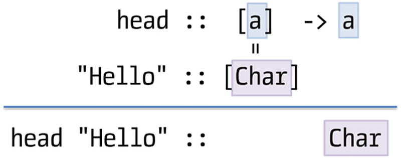
The first function you will look at is foldr, which introduces you to the world of folds. A fold over a data structure such as a list is a function that aggregates or combines all the values contained in that structure to produce a single result. Folds are an expressive and powerful tool, often underestimated. Examples of folds are summing all integers in a list and finding the maximum of the values in the nodes of a tree (I will speak more about trees later).

The definition of foldr includes three arguments: a binary function f that is used to combine elements step-by-step, the initial value for starting aggregation, and finally the list itself.
foldr :: (a -> b -> b) -> b -> [a] -> b
foldr f initial []     = initial
foldr f initial (x:xs) = f x (foldr f initial xs)
This initial value plus binary operation is a common pattern in Haskell code. Usually, the initial value is chosen in such a way that using it as an argument in the binary operation doesn’t change the result. We call such a value a neutral or identity element of the operation. Take, for example, the task of summing all the elements in a list. The chosen operation should intuitively be addition, (+). Then, the initial value should be chosen so as not to affect that operation, and you should now ideally be thinking in terms of the value 0. Let’s follow the evaluation of a call to foldr that exactly performs that task of summing all the elements in a list.
foldr (+) 0 [1,2,3] => 1 + foldr (+) 0 [2,3]
                    => 1 + (2 + foldr (+) [3])
                    => 1 + (2 + (3 + foldr (+) 0 []))
                    => 1 + (2 + (3 + 0))
                    => 1 + (2 + 3) => 1 + 5 => 6
As you can see, foldr traverses the list element by element until it reaches the end. At that moment, foldr uses the initial value to start evaluating the whole call stack that has been created, from the end up to the first application of the corresponding combining function, in this case (+). If you look at a list as a combination of (:) and [] constructors, you can rephrase the algorithm as follows: foldr replaces all instances of (:) by f and all occurrences of [] by the initial value. Figure 3-2 illustrates this thinking.
../images/316945_2_En_3_Chapter/316945_2_En_3_Fig2_HTML.jpg
Figure 3-2

Visual description of foldr

Another example of fold is maximum, which finds the largest value from a list. In this case, the initial value is a bit more elusive because you must consider what the maximum of an empty list is. To help in answering that question, you need to recall the other property that is wanted for the initial value: it should not change the outcome of the binary operation, which in this case is max. This means you have to find a value z such that max(z,x) = max(x,z) = x any value x. You can check that the value that satisfies that property is negative infinity (-∞).

By default, Haskell integers don’t allow representing infinite values, so you need to define a custom data type for this matter. After some thought, you find that the concept of adding infinity values is not unique to integers. The concept also applies to ratios, floating-point values, and so forth. To make the new type more useful, you can define the InfNumber data type as being polymorphic.
data InfNumber a = MinusInfinity
                 | Number a
                 | PlusInfinity
                 deriving Show

By making the type polymorphic, you allow for the possibility of using the type for more than just integers. The immediate problem requires just infinite integer values, but future problems might require, say, infinite floating-point values. Polymorphism here is an investment in the future.

The next step is defining a new binary operation, infMax, to combine two of these numbers.
infMax MinusInfinity x       = x
infMax x MinusInfinity       = x
infMax PlusInfinity  _       = PlusInfinity
infMax _  PlusInfinity       = PlusInfinity
infMax (Number a) (Number b) = Number (max a b)
Let’s try to write the fold.
*Chapter3.Lists> foldr infMax MinusInfinity [1,2,3]
    No instance for (Ord t0) arising from a use of `infMax'
Clearly, it’s not done yet. You are getting an error because the expression that has been written doesn’t pass the type checker. The operation infMax combines elements of type InfNumber, but [1,2,3] is a list of integers. A first solution is to convert the list to InfNumbers by mapping the Number constructor over the list.
*Chapter3.Lists> foldr infMax MinusInfinity $ map Number [1,2,3]
Number 3
However, if you look carefully at the type of foldr, you will see that there’s no need for the combining function (the f argument in foldr) to take values of the same type because it’s not of type a -> a -> a. Rather, the type is a -> b -> b, which means that f should take as the first parameter a value of the type contained in the list, and the second should be the one of the type you are accumulating, which coincides with the type of the initial value (called initial in the definition of foldr shown here). In this case, this means the aggregation function should have type Integer -> InfNumber Integer -> InfNumber Integer since the initial value is MinusInfinity :: InfNumber Integer. You already know how to convert existing numbers into InfNumbers, which is the only special thing you need in the fold.
*Chapter3.Lists> foldr (x y -> infMax (Number x) y) MinusInfinity [1,2,3]
Number 3
The name foldr is a reminder of the algorithm the function implements. It is a fold that associates to the right. That is, the innermost parenthesis will be found on the right side of the expression. Similarly, you can build a fold that associates to the left, which is included in the Haskell Platform as foldl.
foldl :: (a -> b -> a) -> a -> [b] -> a
foldl _ initial [] = initial
foldl f initial (x:xs) = foldl f (f initial x) xs
The innermost parentheses are now at the left, as this evaluation trace shows:
foldl (+) 0 [1,2,3] => foldl (+) (0 + 1) [2,3]
                    => foldl (+) ((0 + 1) + 2) [3]
                    => foldl (+) (((0 + 1) + 2) + 3) []
                    => ((0 + 1) + 2) + 3
                    => (1 + 2) + 3
                    => 3 + 3 => 6

The result value of the fold in the examples so far does not depend on whether it is performed to the right or to the left . But for this to hold, the aggregation operator that is chosen must be commutative. In other words, the following must hold true: f(x,y) = f(y,x)f(x, y) = f(y, x). So long as the order in which parameters are input does not matter, you can make it so that folding left or right also does not matter.

Some operations cannot be made commutative. Subtraction, for example, is not commutative, so the result changes between folds.
*Chapter3.Lists> foldr (-) 0 [1,2,3]
2
*Chapter3.Lists> foldl (-) 0 [1,2,3]
-6
One last version of folds is the one composed of those that do not take an initial value, namely, foldr1 and foldl1. In those, the starting value is the last element (in foldr1) or the first element (in foldl1) of the list. If you know any language derived from Lisp, such as Common Lisp, Racket, or Clojure, you will know this folding operation as reduce. It is not used much in Haskell, but it may come in handy in cases where handling the empty list case is guaranteed not to happen and where handling it tangles the code. As an example, the previously defined maximum function is much easier using foldr1.
maximum' :: [Integer] -> Integer
maximum' = foldr1 max

Exercise 3-3. Your First Folds

Consider the functions product, minimumClient, and all. The product function computes the product of a list of integers. The minimumClient function computes the Client with the shortest name. Finally, the all function computes the conjunction (&&) of a list of Boolean values. Given these functions, do the following:
  • Write the functions using pattern matching, without resorting to any higher-order function.

  • Write the functions as folds. In each case, first try to find the aggregation operation and from that derive a sensible initial value.

Can you find the structure that all these functions share when written in the first style? In which cases is it true that using foldr and foldl give the same results?

Extra: Try to write a minimumBy function such that the order is taken by first applying a function g on the result. For example, minimumBy (x -> -x) [1,2,3] should return 3.

Lists and Predicates

Another big family of list functions comprise those that take Boolean predicates, that is, functions with the type a -> Bool. The filter function I’ve already talked about is a representative of this family. I have already asked you to write the dual version of filter, which only takes elements from a list that doesn’t fulfill a condition. One often needs to group the members of a list depending on whether they satisfy a condition. A naïve way to do this would be as follows:
bothFilters :: (a -> Bool) -> [a] -> ([a],[a])
bothFilters p list = (filter p list, filter (not . p) list)
This definition is correct but has a problem: it will traverse the whole list twice. Intuitively, just one pass should suffice. Haskell defines a function partition inside the Data.List module just for that matter: splitting a list in just one go.
*Chapter3.Lists> import Data.List
*Chapter3.Lists Data.List> partition (> 0) [1,2,-3,4,-5,-6]
([1,2,4],[-3,-5,-6])
If you want to get only the first element in the list that satisfies the condition, you should use find instead of filter. There’s the chance that the list contains no such element. For that reason, find returns a Maybe value.
*Chapter3.Lists Data.List> find (> 0) [1,2,-3,4,-5,-6]
Just 1
*Chapter3.Lists Data.List> find (> 7) [1,2,-3,4,-5,-6]
Nothing
Let’s now move to the following use case: you have a processing system for the shop, with a queue for the clients, which is itself represented as a list where the head is the next client to be served. At high load times, you want to impose the following policy: skip all the clients that are not government organizations. The Data.List module provides a dropWhile function that returns some list from the point in which some predicate becomes false.
skipUntilGov :: [Client a] -> [Client a]
skipUntilGov = dropWhile (case { GovOrg {} -> False ; _ -> True })

Note

Remember you need to enable the LambdaCase extension for the previous code to be accepted by GHC.

Its counterpart is takeWhile, which takes the initial elements until the predicate becomes false. You can use takeWhile to get a list of all the commands in a list until one equals "stop", at which point you quit processing. Here’s the code to do that:
*Chapter3.Lists Data.List> let lst = ["hello", "send", "stop", "receive"]
*Chapter3.Lists Data.List> takeWhile (/= "stop") lst
["hello","send"]
The takeWhile and dropWhile functions are the two components of the function span, which returns both the taken list and the dropped list:
*Chapter3.Lists Data.List> span (/= "stop") lst
(["hello","send"],["stop","receive"])

A related function is break, which does the same work as span but negates the predicate before. Actually, break could be defined as span (not . p).

The last couple of functions that take unary predicates are any and all. As their names suggest, they check whether at least one or all the elements of the list, respectively, fulfill some condition. They are similar to the logical quantifiers “exists” (∃) and “for all” (∀). For example, in the monthly analytics you may want to be sure you have an individual registered in the web shop and that you have at least a company or government organization in the system, that is, some Client that is not an Individual. You may define an -->isIndividual function to start.
isIndividual :: Client a -> Bool
isIndividual (Individual {}) = True
isIndividual _               = False
checkAnalytics :: [Client a] -> (Bool, Bool)
checkAnalytics cs = (any isIndividual cs, not $ all isIndividual cs)
Now let’s move to another kind of predicate: binary ones. These are functions that take two arguments and return some Boolean value by comparing them somehow. The first kind of comparison you can do is whether two elements are equivalent (or not): (==) and (/=) belong to that family. And those are the kind of predicates that the function nubBy expects: it takes out elements such that no two elements in the returned list are equivalent. In this example, you get only one representative of each parity.
*Chapter3.Lists Data.List> let p x y = (even x && even y)||(odd x && odd y)
*Chapter3.Lists Data.List> nubBy p [1,2,3,4,5]
[1,2]
If you use (==) in nubBy, you are essentially removing duplicates in the list.
*Chapter3.Lists Data.List> nubBy (==) [1,2,1,1,3,2,4,1]
[1,2,3,4]
In many cases, types come equipped with a default comparison. You will see how to add that default comparison to your own types in the next chapter, when I talk about type classes. If the values support it, like those of the Integer type, you can just use nub and drop the equivalence function.
*Chapter3.Lists Data.List> nub [1,2,1,1,3,2,4,1]
[1,2,3,4]

Note

nub and nubBy are not very performant functions because they must check for equality between all possible pairs of elements. This means the order of the function is quadratic. In the next chapter, you will learn a faster way to remove duplicates from a list.

Equality checks, or more broadly equivalence checks, can be used to maintain lists as sets: holding only a copy of each value. The main functions are union(By), which returns a new set with all the elements from the initial ones; intersect(By), which returns a set holding only the elements in both sets; insert(By), which adds only one element to a set; and (\), which performs the difference between sets: x1 \ x2 contains all elements in x1 that are not in x2. In each case, the version ending in By takes a parameter telling how to check elements for equivalence, whereas the other versions use the default comparison.
*Chapter3.Lists Data.List> :{
*Chapter3.Lists Data.List | let x1 = [1,2,3,4]
*Chapter3.Lists Data.List |     x2 = [2,3,5]
*Chapter3.Lists Data.List | in (x1 `union` x2, x1 `intersect` x2, x1 \ x2)
*Chapter3.Lists Data.List | :}
([1,2,3,4,5],[2,3],[1,4])

This example also shows an interesting feature of Haskell syntax: infix notation. Each time you have a two-argument function that doesn’t have a name made only of symbols (such as union or intersect), you can write the name between the arguments surrounding it by back quotes, ``.

Finally, elem just points out whether an element is a member of a list.
*Chapter3.Lists Data.List> 2 `elem` [1,2,3]
True
*Chapter3.Lists Data.List> 4 `elem` [1,2,3]
False

Mini-exercise

Write elem using find and pattern matching.

The other usual meaning for binary predicates is ordering: p x y means that in some way x precedes y. However, for both clarity and performance reasons, ordering in Haskell is not defined by returning a Bool but by returning an Ordering value, which can be LT (less than), EQ (equal), or GT (greater than). For example, you can define a function representing that companies and government organizations go first in an ordering of clients and individuals are next. In each level, draws are decided by the names of the clients. The following is the code to implement that function, and it is written knowing that the built-in compare function defines an Ordering for strings:
compareClient :: Client a -> Client a -> Ordering
compareClient (Individual{person = p1}) (Individual{person = p2})
                                = compare (firstName p1) (firstName p2)
compareClient (Individual {}) _ = GT
compareClient _ (Individual {}) = LT
compareClient c1 c2             = compare (clientName c1) (clientName c2)
In the following examples, the code will use part of my list of clients. As you may suspect, many of the popular scientists, writers, and adventurers of the time buy or read books in the store.
listOfClients
  = [ Individual 2 (Person "H. G." "Wells")
    , GovOrg 3 "NTTF"  -- National Time Travel Foundation
    , Company 4 "Wormhole Inc." (Person "Karl" "Schwarzschild") "Physicist"
    , Individual 5 (Person "Doctor" "")
    , Individual 6 (Person "Sarah" "Jane")
    ]
Using the auxiliary function named compareClient, you can sort a whole list of Clients using sortBy.
*Chapter3.Lists Data.List> sortBy compareClient listOfClients
[ GovOrg { clientId = 3, clientName = "NTTF" }
, Company { clientId = 4, clientName = "Wormhole Inc."
          , person = Person { firstName = "Karl"
                            , lastName = "Schwarzschild" }
          , duty = "Physicist"}
, Individual { clientId = 5, person = Person { firstName = "Doctor"
                                             , lastName = "" }}
, Individual { clientId = 2, person = Person { firstName = "H. G."
                                             , lastName = "Wells" }}
, Individual { clientId = 6, person = Person { firstName = "Sarah"
                                             , lastName = "Jane" }} ]
Some types already come defined with a default way in which to order values. Numbers and characters are examples of such types, which are readily compared. In those cases, you can invoke the function sort, which doesn’t need a comparison function. Here’s an example:
*Chapter3.Lists Data.List> sort [1,4,2,-3]
[-3,1,2,4]
It’s interesting to see that orders are also defined for tuples and lists if their contained elements have a default comparison. In both cases, this order is lexicographic: values are compared element by element. Lexicographic comparison means that if the first component of the tuples is different, then the ordering of those two values decides the ordering of the tuple. If the leading values match, the second elements are compared, and so on. The same approach is taken for lists as with tuples. Also, for lists, a smaller list is considered previous in order to a longer list that contains the shorter list as a prefix. Let’s look at same examples of comparison that clearly show this lexicographic comparison. In the first and third cases, tuples or lists are equal up to some point, whereas in the second case the first list is shorter than the second one.
*Chapter3.Lists> compare (1,2) (1,1)
GT
*Chapter3.Lists> compare "Hello" "Hello world
LT
*Chapter3.Lists> compare "This" "That"
GT
When a compare function is defined, Haskell also provides implementations of the (>), (<), (>=), and (<=) operators. These operators usually help clarify the code that you write because you don’t need to call compare and then pattern match on the output. Furthermore, these operators are more familiar. The previous example could have been expressed also using (<=), as follows. Notice that this operator returns a simple Boolean instead of a value of the Ordering type.
*Chapter3.Lists> (1,2) <= (1,1)
False
*Chapter3.Lists> "Hello" <= "Hello world"
True
*Chapter3.Lists> "This" <= "That"
False

It may become handy when performing analytics to group clients depending on some characteristic. The function groupBy, with type (a -> a -> Bool) -> [a] -> [[a]], puts in a single list all those elements for which the equivalence predicate returns True; that is, they must be in the same group.

For example, you would like to find out which company duties are the most common in the database (which right now is just a list). To find this out, you can first filter out those elements that are not companies, using filter. Then, you can group the clients depending on their duty (the comparison function to groupBy). A third step would be sorting the lists depending on their length. While sorting, keep in mind that if you want to have the most common duty first, you need to sort the list lengths in reverse order; you need the longest list first. Finally, you retrieve the duty from each list by accessing the head element. You can do so safely because all lists will be nonempty. You also know that all elements in a given list will share the same duty, so any element that you access is as good as any other. The resulting function to do all this would be as follows:
companyDutiesAnalytics :: [Client a] -> [String]
companyDutiesAnalytics = map (duty . head) .
                           sortBy (x y -> compare (length y) (length x)) .
                           groupBy (x y -> duty x == duty y) .
                           filter isCompany
                         where isCompany (Company {}) = True
                               isCompany _            = False
There’s a more elegant way to write this function. As you can see, there’s a pattern in which two elements are compared but only after applying some operation to the values. The higher-order function on, in the module Data.Function, allows composing the comparison and the value-extracting functions as you want, as the following code illustrates. To reverse the ordering for list lengths, a useful trick is calling the comparison function with the arguments in the reverse order. There’s a combinator specifically designed for calling a two-parameter function with the arguments reversed, which is called flip :: (a -> b -> c) -> (b -> a -> c). The following code is a point-free version of the previous one:
companyDutiesAnalytics :: [Client a] -> [String]
companyDutiesAnalytics = map (duty . head) .
                           sortBy (flip  (compare `on` length)) .
                           groupBy ((==) `on` duty) .
                           filter isCompany
                         where isCompany (Company {}) = True
                               isCompany _            = False

Haskell is Declarative

You may wonder why Haskell provides so many different functions on lists, whereas other programming languages do fine with constructs such as iterators or for loops. The idea is that instead of explicitly transforming a list element by element, you declare transformations at a higher level of abstraction. Languages supporting this idea, such as Haskell, are called declarative.

A classical fear when programming in Haskell is that this higher level of abstraction hurts performance. However, compilers of declarative languages are able to apply a wider range of optimizations because they can change the code in many more ways while retaining the same behavior. A typical example takes the form map f . map g. This code performs multiple passes over the data but can safely be converted by the compiler to map (f . g), which performs the same duty in just one pass over the data.

Lists Containing Tuples

Another family of list functions is the one that considers lists that have tuples inside. These list types will all ultimately be founded on some instance of the type [(a,b)]. I’ve already mentioned that default comparisons work on tuples lexicographically. Set functions such as nub and sorting functions such as sort work in that same way.

Previously in the book you wrote a function converting two lists into a list of tuples. This function is known as zip because it interleaves elements like a zipper does. One use of zip is to include the position of each element next to the element itself. For example, applying zip to ['a', 'b', 'c'] would give you [(1,'a'),(2,'b'),(3,'c')]. This involves zipping the original list with a list from the number 1 to the length of the list itself. Picture two sides of a zipper, one corresponding to the list of numbers and the second to the list of characters. As you pull up the fastener, each number is associated to a character, one by one.

As an example, let’s define a function enum that generates a list of numbers.
enum :: Int -> Int -> [Int]
enum a b | a > b = []
enum a b         = a : enum (a+1) b
The length function in Prelude returns the number of elements contained in a list. With these two ingredients, you can build the function you want.
withPositions :: [a] -> [(Int,a)]
withPositions list = zip (enum 1 $ length list) list
There is a special way to construct lists for types that have a default ordering, such as integers or characters. This is called a range and has the syntax [ a .. b ] to get a list with all elements in between and including a and b. For example, you can substitute the function enum as shown here:
withPositions list = zip [1 .. length list] list
There is an unzip function that does the reverse of zip and gets two lists back from a list of tuples. For example, let’s split countries and their capitals from a list of pairs.
*Chapter3.Lists> unzip [("France","Paris"),("Spain","Madrid"),("Portugal","Lisbon")]
(["France","Spain","Portugal"],["Paris","Madrid","Lisbon"])
This last example shows one possible use of a list of tuples: to implement a mapping between keys and values. A list of such characteristics is called an association list and is a well-known structure in functional programming. The function named lookup enables searching for the value associated with a particular key. Once again, the possibility of not finding the key implies that the returned value is wrapped on a Maybe.3
*Chapter3.Lists> lookup "Spain" [("France","Paris"),("Spain","Madrid"),("Portugal","Lisbon")]
Just "Madrid"
*Chapter3.Lists> lookup "UK" [("France","Paris"),("Spain","Madrid"),("Portugal","Lisbon")]
Nothing

Caution

You have seen how a list can be used to represent sets and maps. However, those implementations are inefficient because they require traversing a list for most operations. In the next chapter, you will look at other containers such as those found in the modules Data.Set and Data.Map. These other containers are especially suited for their particular uses and have highly performant implementations.

List Comprehensions

The fact that so many list functions are included in the standard library, and most of them even in Prelude (and hence available by default in any Haskell source), highlights the importance of lists in functional programming. You have seen how function composition allows for a very declarative programming style, where transformations are defined by steps. Remember the function duplicateOdds for computing the double of all odd numbers in list is written as follows:
duplicateOdds :: [Integer] -> [Integer]
duplicateOdds list = map (*2) $ filter odd list
However, if you remember your algebra classes, mathematicians have a terse but intuitive language for manipulating sets. The previous example can be written in set notation as {2x| x ∈ list. odd(x)}. The Haskell designers also like this syntax, so they included list comprehensions to mimic it. The example becomes the following:
duplicateOdds list = [ 2 * x | x <- list, odd x ]

List comprehensions have two parts, separated by | and wrapped by square brackets. The first part is the expression, which defines a transformation to apply to all the elements that will be returned. The second part consists a list of qualifiers and specifies from whence the elements will come and the constraints upon them.

The first kind of qualifiers are generators, which take the form e <- list. Generators indicate that elements from list will be acted upon, and each of the elements will be referred as e in the rest of the comprehension. Optionally, the e part can be a pattern, stating that only values matching it will be included. For example, you can get the client names of all government organizations using this:
*Chapter3.Compr> [ clientName x | x@(GovOrg _ _) <- listOfClients ]
["NTTF"]
A list comprehension may have multiple generators. The simplest way to implement multiple generators is to iterate in two different lists without any relationship between them and get all possible combinations of elements coming from each list. This result of all possible combinations is called the product of those lists. As an example, the following code applies the product of two lists to the problem of generating the multiplication tables from 1 to 4:
*Chapter3.Compr> [(x,y,x*y) | x <- [1 .. 4], y <- [1 .. 10]]
[(1,1,1),(1,2,2),(1,3,3),(1,4,4),(1,5,5),(1,6,6),(1,7,7),(1,8,8),(1,9,9),(1,10,10),(2,1,2),(2,2,4),(2,3,6),(2,4,8),(2,5,10),(2,6,12),(2,7,14),(2,8,16),(2,9,18),(2,10,20),(3,1,3),(3,2,6),(3,3,9),(3,4,12),(3,5,15),(3,6,18),(3,7,21),(3,8,24),(3,9,27),(3,10,30),(4,1,4),(4,2,8),(4,3,12),(4,4,16),(4,5,20),(4,6,24),(4,7,28),(4,8,32),(4,9,36),(4,10,40)]
But a generator may also depend on other values in the comprehension, in particular on an element from another generator. For example, you may want to enumerate all possible dominoes. But you know that once you have (1,6), the piece (6,1) is exactly the same, so you shouldn’t show that one. A way to get the correct result is, for each first component in the list of dominoes, get only values equal or greater than that in the second component. Thus, a result of (6,1) is excluded, because 1 is less than 6. Here’s some code to implement that approach:
*Chapter3.Compr> [(x,y) | x <- [0 .. 6], y <- [x .. 6]] [(0,0),(0,1),(0,2),(0,3),(0,4),(0,5),(0,6), (1,1),(1,2),(1,3),(1,4),(1,5),(1,6),
(2,2),(2,3),(2,4),(2,5),(2,6),
(3,3),(3,4),(3,5),(3,6),
(4,4),(4,5),(4,6),
(5,5),(5,6),
(6,6)]
Finally, an element in a list may itself be a list, which allows it to appear on the right side of the generator. Given a list of words (remember that a string is itself a list of characters), you can concatenate all of them and show them in uppercase by iterating twice.
*Chapter3.Compr> import Data.Char
*Chapter3.Compr Data.Char> [ toUpper c | s <- "A","list"], c <- ' ':s ]
" A LIST"
Sometimes you want to introduce local bindings inside a comprehension, usually to enhance the readability of the code. This second form of qualifiers has a syntax that is similar to that in expressions, and the form is let b = expression. For example, you may be interested in computing the norms of a list of vectors represented as tuples.4
*Chapter3.Compr> [ sqrt v | (x,y) <- [(1,2),(3,8)], let v = x*x+y*y ]
[2.23606797749979,8.54400374531753]
Finally, list comprehensions allow filtering out some elements using a guard. Guards are the third form of qualifiers and are syntactically just a call to a predicate. Only those elements satisfying the guard will go in the returned list. Guards allow expressing the invariant for dominoes in a different way.
*Chapter3.Compr> [(x,y) | x <- [1 .. 6], y <- [1 .. 6], x <= y]
[(1,1),(1,2),(1,3),(1,4),(1,5),(1,6),(2,2),(2,3),(2,4),(2,5),(2,6),
(3,3),(3,4),(3,5),(3,6),(4,4),(4,5),(4,6),(5,5),(5,6),(6,6)]

Note

If you know Scala, list comprehensions in Haskell will be familiar to you. The changes are merely syntactic: [ e | q ] becomes for (q) yield e;, and the generators are written the same. Local bindings are introduced without any keyword, whereas guards must be preceded by if.

You have looked at comprehensions as coming from mathematical notation for sets. But if you look closer, they also look a bit like SQL. The notation [ x | x <- list, b x ] can be seen in SQL as select x from list where b=x. However, if you want to have a full-fledged query language, you need also grouping and sorting. The great news is that GHC already provides those operations; you need only to enable the TransformListComp extension.

The first qualifier that is provided by the TransformListComp extension is then. A qualifier then f transforms the input list by applying the function f to the result of the comprehension up to that point. The constraint is that f should have type [a] -> [a], so its applicability is a bit limited. Nevertheless, you can use it to reverse a list at the end.
*Chapter3.Compr> :set -XTransformListComp
*Chapter3.Compr> [x*y | x <- [-1,1,-2], y <- [1,2,3], then reverse]
[-6,-4,-2,3,2,1,-3,-2,-1]
A more powerful enhancement is then f by e, which must transform the list depending on some expression. The most common use is to sort a list. To do so, you first need to import the module GHC.Exts, which contains the function sortWith. Now, include the qualifier then sortWith by v to sort depending on the values in v. You may decide to return the previous list but now ordered by the values of x.
*Chapter3.Compr> import GHC.Exts
*Chapter3.Compr GHC.Exts> :{
*Chapter3.Compr GHC.Exts| [x*y | x <- [-1,1,-2], y <- [1,2,3]
*Chapter3.Compr GHC.Exts|      , then sortWith by x]
*Chapter3.Compr GHC.Exts| :}
[-2,-4,-6,-1,-2,-3,1,2,3]

The final extension concerns grouping. The syntax is then group by e using f, where f is a function of the type (a -> b) -> [a] -> [[a]]. In the most common case, you use as groupWith, also in GHC.Exts, which computes e for each element in the list and groups together those values for which e returns the same result. After a grouping qualifier, all the previous bindings are considered to be lists made up of the previous elements. This is important because all the transformations to the grouped elements should be done prior to that point. In many cases, all grouped elements will be equal, so GHC provides a the function that takes just one element from the list.

For example, you can group the numbers from the previous example according to whether they are positive.
*Chapter3.Compr GHC.Exts> :{
*Chapter3.Compr GHC.Exts| [ (the p, m) | x <- [-1,1,-2]
*Chapter3.Compr GHC.Exts|              , y <- [1,2,3]
*Chapter3.Compr GHC.Exts|              , let m = x*y
*Chapter3.Compr GHC.Exts|              , let p = m > 0
*Chapter3.Compr GHC.Exts|              , then group by p using groupWith ]
*Chapter3.Compr GHC.Exts| :}
 [(False,[-1,-2,-3,-2,-4,-6]),(True,[1,2,3])]

Notice how this code computes the product of the items before the grouping using let m = x*y. Then you group according to the value m > 0, and at this point you have the list [([False,False,False,False,False,False],[-1,-2,-3,-2,-4,-6]),([True,True,True],[1,2,3])]. Finally, you apply the to conflate the first components to a single element.

To help you understand these ideas about list comprehensions, let’s try to build a comprehension to analyze your enterprise clients. As you may remember, you can have more than one person from each company in the database. The idea is to group all the records belonging to the same company sorted by duty and then to sort the companies by the number of records. The following code accomplishes those goals:
companyAnalytics :: [Client a] -> [(String, [(Person, String)])]
companyAnalytics clients = [ (the clientName, zip person duty)
                           | client@(Company { .. }) <- clients
                           , then sortWith by duty
                           , then group by clientName using groupWith
                           , then sortWith by length client
                           ]

Note

These comprehensions resemble the query expressions introduced in the C# language in version 3.0.

GHC supports another extension, parallel comprehension, which performs a duty that is not found in SQL queries: traversing several lists at the same time. The extension is enabled via the ParallelListComp pragma. Using this functionality, more than one branch of qualifiers can be stated in the comprehension, each of them separated by |. Instead of performing nested iterations, the result of all the branches will be zipped and available for the expression. Here’s an example where you perform the multiplication of pairs of numbers, each component being given in a different list. Compare the result when using traditional nesting and when zipping.
*Chapter3.Compr> :set -XParallelListComp
*Chapter3.Compr> [ x*y | x <- [1,2,3], y <- [1,2,3] ]   -- nesting
[1,2,3,2,4,6,3,6,9]
*Chapter3.Compr> [ x*y | x <- [1,2,3] | y <- [1,2,3] ]  -- zipping
[1,4,9]

Haskell Origami

Origami is the Japanese art of folding and unfolding paper in order to create beautiful pieces of art. You have already looked at list folds. In this section you will look at them and meet their colleagues, the unfolds. The goal is gaining some deeper understanding of the structure of list functions and how this huge set of functions I have described can be fit into a small family of schemas. Since these schemas are based on fold and unfold functions, they are known as Haskell origami . This section contains some optional and more advanced material. Don’t worry if you don’t understand this upon first read; just come try it again after some time.5

Let’s start with an observation: folds are much more powerful than you imagine. You can write almost all list functions using foldr. For example, you can write filter as a fold by accumulating values on a list.
filterAsFold :: (a -> Bool) -> [a] -> [a]
filterAsFold p = foldr (x l -> if p x then x : l else l) []

But, how to ensure that the definition of filter using regular pattern matching and recursion on lists and this definition using a fold are equivalent? The answer lies in induction and equational reasoning, a technique for formally verifying code that manipulates equations between functions. In this particular case, you need to prove that both ways to define filtering work in the same way for the empty list (this is called the base case) and that by assuming that they are equal for a list xs you can prove that they are equal for a longer list x:xs (this is called the inductive step).

Remapping our landscape, we want to prove that filter p xs is equal to filterAsFold p xs for any list xs. We start by considering the base case, in which we make xs = []. By the definition of the function, filter p [] = []. For the other side, we can write the following set of equalities:
filterAsFold p [] = foldr (x l -> if p x then x : l else l) [] []
                  = []  -- we get back the initial value
Since both expressions give us the same result, they must be equal among themselves. Now for the inductive step, we need to consider a list of the form x:xs.
filter p (x:xs) = if p x
                  then x : filter p xs
                  else     filter p xs
filterAsFold p (x:xs) = foldr (x l -> if p x then x : l else l) [] (x:xs)
                      = (x l -> if p x then x : l else l)
                         x (foldr (x l -> if p x then x : l else l) [] xs)
                      = if p x
                        then x : (foldr (x l -> if p x then x : l else l) [] xs)
                        else     (foldr (x l -> if p x then x : l else l) [] xs)
We can see that the structure of the code is the same. Remember that we are allowed to assume that the equality foldr p xs = filterAsFold p xs holds, let us call this common expression ys. Thus both expressions can be rewritten to:
if p x then x : ys else ys

By induction, the equality between both ways to write the function is now proven, in the mathematical sense of the word.

You can also define map in terms of foldr. Exercise 3-4 asks you to prove that both definitions are equivalent:
mapAsFold :: (a -> b) -> [a] -> [b]
mapAsFold f = foldr (x l -> f x : l) []

Exercise 3-4. Proof For Map

Using the same techniques as we used for filter, prove that the usual map definition and the one given in terms of foldr are equal.

The techniques of induction and equational reasoning are not limited to prove equivalence between different function definitions. We can also state laws which combine several operations. One such law is:
foldr f v . map g = foldr (x xs -> f (g x) xs) v
In that form, this law relates two functions. However, in order to prove their equality, we need to introduce explicit arguments. That is, what we want to hold is that for any input list is,
foldr f v (map g is) = foldr (x xs -> f (g x) xs) v is
At this point, we can start using our techniques. First, we have to prove that the equality holds for the case in which is is the empty list.
foldr f v (map g []) = foldr f v [] = v
foldr (x xs -> f (g x) xs) v is    = v
Since both expressions rewrite to the initial value v, the base case is proven. The inductive step leads us to consider the case in which the list has the form i:is.
foldr f v (map g (i:is)) = foldr f v (g i : map g is)
                         = f (g i) (foldr f v (map g is))
foldr (x xs -> f (g x) xs) v (i:is)
  = (x xs -> f (g x) xs) i (foldr (x xs -> f (g x) xs) v is)
  = f (g i) (foldr (x xs -> f (g x) xs) v is)

As in the case of filter, we see that the final expressions have the same structure. Remember that we can assume that the equality already holds for is while proving the inductive step. If we call such common expression js, in both cases we obtain f (g i) js. The proof is finished.

If you don’t feel completely confident about how I reasoned, try to go step-by-step with pencil and paper. Pay close attention in each step to how you apply the rules of the game. Once you are sure about the details, try to prove the so-called fusion law for maps:
map f . map g = map (f . g).

Note

Knowing these laws may seem like just a theoretical exercise. However, they have important applications for Haskell programs because the compiler uses them to transform the code into a more efficient one, while ensuring the same behavior. For example, map (f . g) traverses a list only once, whereas map f . map g does it twice and needs an intermediate data structure in memory. So, the compiler aims to replace each instance of the latter with the former.

Up to now I have talked about folds, which consume lists to provide a single value. However, there’s a corresponding concept, unfolds, which create lists out of some seed. Like with folds, there are both right and left unfolds. Here, the focus will be on the right unfold function unfoldr, which is available in Data.List. Let’s begin looking at its type.
*Chapter3.Origami Data.List> :t unfoldr
unfoldr :: (b -> Maybe (a, b)) -> b -> [a]
The algorithm for unfolding is the following: start with a seed of type b. Apply the function given as the first argument. You can get two kinds of output: Nothing signals that unfoldr should stop producing elements, whereas Just (x, s) attaches x to the new list and continues the process with a new seed, s. For example, let’s create a list from n to m. The function should produce a number in each step and increase it for the next iteration, and it should stop when the seed is larger than m. Here’s the code to do this:
enumUnfold :: Int -> Int -> [Int]
enumUnfold n m = unfoldr (x -> if x > m then Nothing else Just (x, x+1)) n
Figure 3-3 illustrates the step-by-step execution of this code.
../images/316945_2_En_3_Chapter/316945_2_En_3_Fig3_HTML.jpg
Figure 3-3

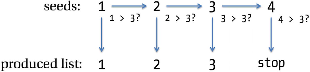
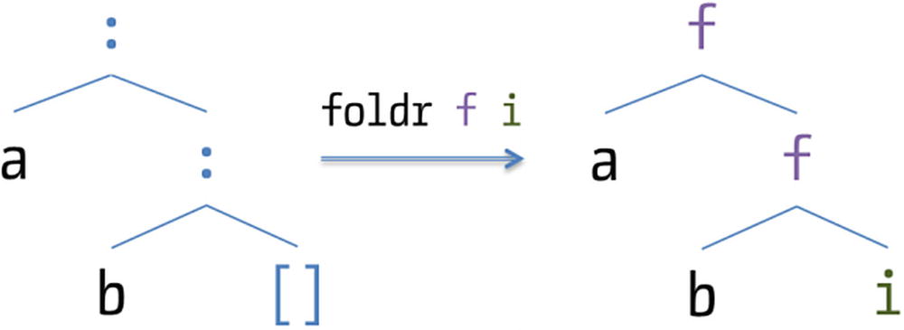
Evaluation steps for enumUnfold 1 3

Another algorithm that can be expressed as an unfold is minimum sort for lists. In minimum sort, you make a series of steps, and in each one you find the minimum element in the input list, take it out of this input list, and add it to the output list, which will end sorted. To implement it as an unfold, you will use a list as the seed, containing the elements that are yet to be ordered. In each step, take the minimum element from the list, making the new seed the previous list without that element. When you have an empty list as a seed, you should stop generating new elements. Here it is in Haskell code:
minSort :: [Integer] -> [Integer]
minSort = unfoldr (case [] -> Nothing
                         xs -> Just (m, delete m xs) where m = minimum xs)

Why Are Folds And Unfolds Duals?

The two concepts of folding and unfolding are dual, but how do I back up that claim? The key point is that unfoldr returns eithers Nothing for stopping or Just for continuing, whereas foldr takes different arguments for the empty and general cases. You can group the initial value and combination function into a single function of type Maybe (a,b) -> b, which will return the initial value if given nothing or apply the combination for Just.
{-# LANGUAGE LambdaCase #-}
foldr2 :: (Maybe (a,b) -> b) -> [a] -> b
foldr2 f []     = f Nothing
foldr2 f (x:xs) = f $ Just (x, foldr2 f xs)
mapAsFold2 :: (a -> b) -> [a] -> [b]
mapAsFold2 f = foldr2 (case Nothing     -> []
                             Just (x,xs) -> f x : xs)
Now you can see how the two functions have reflected types.
foldr2  :: (Maybe (a,b) -> b) -> [a] -> b
unfoldr :: (b -> (Maybe (a,b)) -> b -> [a]

I find this duality elegant and an example of how higher-order functions allow you to find relations between different abstractions.

Summary

The chapter covered many concepts related to reusability and lists. It finished with a look at list origami.
  • You got in touch with the idea of parametric polymorphism, which allows you to define functions operating on several types and also write data types that may contain values of different types.

  • You learned how to use functions as parameters or return values, giving rise to higher-order functions, which greatly enhance the reusability of your code.

  • Anonymous functions were introduced as a way to write some code directly in place instead of having to define a new function each time you want to pass it as an argument.

  • You saw how the idea of functions returning functions permeates the Haskell language and saw the syntax for partially applying them.

  • You looked at the point-free programming style, which encourages the use of combinators between functions to write more concise code. In particular, the focus was on the (.) composition operator.

  • The chapter covered the import and export of definitions in other modules in a project. In particular, you saw how hiding definitions allows for the smart constructors pattern.

  • You walked through the most important functions in the Data.List module, introducing the important concept of a fold.

  • In many cases, list comprehensions provide an intuitive syntax for list transformations. You delved into its basic characteristics and the particular GHC extensions providing sorting and grouping à la SQL.

  • Finally, you saw how fold and unfolds are at the core of most list functions, and you learned how to use them and reason with them.

..................Content has been hidden....................

You can't read the all page of ebook, please click here login for view all page.
Reset
18.119.164.176