© Alejandro Serrano Mena 2019
Alejandro Serrano MenaPractical Haskellhttps://doi.org/10.1007/978-1-4842-4480-7_6

6. Knowing Your Clients Using Monads

Alejandro Serrano Mena1 
(1)
Utrecht, The Netherlands
 

Remember that you have been commissioned to build a Time Machine Store. Apart from a beautiful design and an intuitive user experience, a good web store should adapt itself to the customers’ likes and needs by keeping track of clients and analyzing their behavior. With that information, better campaigns, such as discounts or targeted ads, can be developed, increasing sales. For these tasks, many data-mining algorithms have been developed. In this chapter you will focus on clustering algorithms, which try to find groups of related clients. You will use a specific implementation of clustering, called K-means, using Haskell.

The K-means algorithm is better understood in terms of a set of vectors. Each vector is an aggregation of numeric variables describing a client, product, or purchase, and each vector changes in every iteration. In an imperative language, these vectors would be modeled as a set of variables that are updated in a loop. The solution presented in this chapter will start with a basic implementation where you will keep track of all the information. I’ll then introduce lenses, which are used to manipulate and query data structures in a concise way; you’ll refine the code and split it into a set of basic combinators that glue together the different parts.

Looking at those combinators and their relation to other data types will lead to the notion of monad, one of the central idioms (and type classes) in Haskell code. You will explore its definition and laws and compare it to the other pervasive type class, the functor. Many instances of the Monad class are available in the Haskell Platform; in this chapter, I will focus on those related in some way to keeping track of state.

The idea of monad is not complex, but it has enormous ramifications in Haskell. For that reason, both this chapter and the next one are devoted to understanding monads in depth.

Data Mining

Data mining is a wide field and comprises many kinds of algorithms that use statistics, machine learning, and artificial intelligence; data mining is about discovering different patterns in the data. The following are two concrete tasks that you will consider in this chapter and the next:
  • Discovering the different types of clients that use the time machine store, based on their user information and their purchase history. Clustering tries to discern groups (or clusters in data mining jargon) of elements that share common properties. The hope is that, using this information, the marketing team can better target their campaigns.

  • Detecting the purchase habits of each type of client. This will allow you to tailor the discounts (there will be more discussions about discounts in the last part of the book). For that matter, the idea is to learn association rules and later use them to derive conclusions.

    Note Since the store is selling time machines, you could use the machines to travel in time and look at trends in the future. However, this is sort of dishonest, so you should try to use current data and technology to perform better in the market.

Implementing K-means

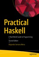
K-means is one of the simplest algorithms for performing clustering on a set of data. The information in this case is represented as a set of points in n-dimensional space, with each of them representing a different observed fact. The similarity between two facts corresponds to the proximity of the points. The concrete task of the algorithm will be dividing the whole set of points into k partitions, such that the aggregated distance of the points in each partition is minimized.

Note

The number of partitions to create is usually represented as k and must be explicitly given as input to the algorithm. This need to specify the number of partitions up front is one of the shortcomings of K-means. Different methods are proposed in the literature to determine the best value to provide. The Wikipedia article at http://en.wikipedia.org/wiki/Determining_the_number_of_clusters_in_a_data_set summarizes the different approaches.

For example, Figure 6-1 shows a set of 2D points. The K-means algorithm has been executed over that set of points with k=3. The output of the algorithm (i.e., the three clusters of points) is distinguished in the figure by a common shape used to draw them. Cluster 1 is drawn with circles, cluster 2 uses triangles, and cluster 3 uses crosses.
../images/316945_2_En_6_Chapter/316945_2_En_6_Fig1_HTML.jpg
Figure 6-1

Clusters obtained for an example data set

This example shows a main characteristic of K-means: it works only on vectors for which you can define a notion of distance and proximity. Another approach would be using a tuple for representing that information, but using a tuple poses the problem that the number of components of the vectors should be constant among all the uses of the algorithm. This is not a reasonable assumption because taking into account some new information (e.g., deciding to cluster also depending on the age) would require changing all the type definitions. Another possibility would be to use lists, but then you lose the safety enforced by tuples (because lists can have different numbers of elements). The best option then is to define a new type class, Vector, which will have as instances all data types supporting the distance operation you need.
class Vector v where
  distance :: v -> v -> Double
The following is one possible implementation for numeric pairs using the Euclidean distance measure:
{-# LANGUAGE FlexibleInstances #-}
instance Vector (Double, Double) where
  distance (a,b) (c,d) = sqrt $ (c-a)*(c-a) + (d-b)*(d-b)

Note

The Haskell Report allows instance declarations only for types whose shape is a name followed by a list of distinct type variables. The previous definition doesn’t follow that lead, so the compiler complains. However, GHC supports those declarations if you enable the FlexibleInstances extension.
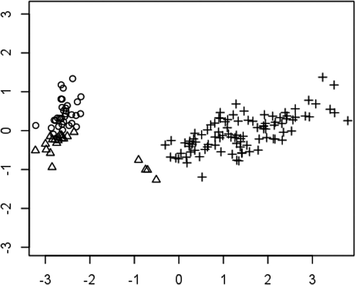
Furthermore, you also need to specify how to translate one item in your data into its corresponding vector. Again, doing so using a type class is the best way to go. But this time you need to specify two types taking part in the type class: the type of the items to convert and the type of the vectors in which they are translated. You can do so by using multiparameter type classes , which follow the same syntax as one-parameter ones, and by enabling the MultiParamTypeClasses extension. However, the concept of type classes with two or more parameters departs from being just like an interface in an object-oriented language and looks more like a contract between two different types. Working with these type classes can be tricky; you will explore the implications of them throughout the book. The name given to elements translatable to vectors will be, no surprise here, Vectorizables. Here’s the definition and a simple instance for performing the identity conversion between Double pairs:
{-# LANGUAGE MultiParamTypeClasses #-}
class Vector v => Vectorizable e v where
  toVector :: e -> v
instance Vectorizable (Double,Double) (Double,Double) where
  toVector = id
The way in which the K-means algorithm describes a cluster is via one vector for each, called the centroid of the cluster. Each element in the data set is assigned to the cluster whose centroid is nearer to the data point. After knowing this fact, you already have an initial idea of how the type of K-means should look.
kMeans :: (Vector v, Vectorizable e v)
       => Int  -- number of centroids
       -> [e]  -- the information
       -> [v]  -- centroids after convergence
The K-means algorithm is simple. In a first phase it generates k vectors, which will be used as the initial centroids. Then, each point is assigned to the cluster of the nearest centroid. In that way, a first partition of the data points is created. After all points have been assigned, the algorithm computes new centroids. The updated centroid of each cluster will be the average of all the points in that cluster. These new centroids will be the input of the new cluster-point assignment and centroid updating phases, and so on. At some point, the clusters will be stable: the partition and the clusters won’t change anymore. Thus, the procedure stops and returns the centroids as the final ones. Figure 6-2 pictures this process as a diagram.
../images/316945_2_En_6_Chapter/316945_2_En_6_Fig2_HTML.png
Figure 6-2

K-means algorithm

Let’s work on each of the steps and finally join everything together into a big algorithm. There are several options for generating the initial vectors. One possibility is generating random vectors; another one is choosing k of the vectors in the data set (this is called the Forgy method). The best option is to abstract this choice and include an extra argument to the kMeans function for the function generating the initial values. The type of the function in this case would turn into this:
kMeans :: (Vector v, Vectorizable e v)
       => (Int -> [e] -> [v]) -> [e] -> [v]

The cluster assignment phase should receive the current centroids and the elements of the set and decide which centroid each element corresponds with. This is done based on the proximity. Since you have a key (cluster) to values (points) mapping, it makes sense to use a Map to hold the assignments. This implies that you need to include an extra Ord v constraint in the Vector type class because Map keys must fulfill that requirement.

This cluster assignment phase can be divided in two different tasks. The first one is creating the Map with all the keys assigned to empty lists. At this point there’s an implicit assumption that no two keys will be the same at any point of the algorithm, but in a more complete implementation this should be taken care of. The second task should go element by element and find the centroid closer to it and then add the element to the list of the chosen centroid. Remember that you must first translate the element to a vector using the toVector function . The following code uses folds both for creating the initial maps and for updating each element in the data set:
import Data.List
import qualified Data.Map as M
clusterAssignmentPhase :: (Ord v, Vector v, Vectorizable e v)
                       => [v] -> [e] -> M.Map v [e]
clusterAssignmentPhase centroids points =
  let initialMap = M.fromList $ zip centroids (repeat [])
   in foldr (p m -> let chosenC = minimumBy (compareDistance p) centroids
                      in M.adjust (p:) chosenC m)
            initialMap points
  where compareDistance p x y = compare (distance x $ toVector p)
                                        (distance y $ toVector p)
Finally, you have to compute the new centroid of each cluster. To do so, you need to map from the elements in a cluster to a vector. You can see now that an extra function was left out in the type class for Vectors: computing the centroid of a set of them. Thus, let’s augment that type class and implement it for Double pairs. We also add Ord v as a superclass of Vector, since it is required by the Map operations.
class Ord v => Vector v where
  distance :: v -> v -> Double
  centroid :: [v] -> v
instance Vector (Double, Double) where
  distance (a,b) (c,d) = sqrt $ (c-a)*(c-a) + (d-b)*(d-b)
  centroid lst = let (u,v) = foldr ((a,b) (c,d) -> (a+c,b+d)) (0,0) lst
                     n = fromIntegral $ length lst
                  in (u / n, v / n)
With this new function, it’s straightforward to implement the computation of new centroids. The idea of the code is the following: for each cluster (so you need to use fmap), convert the list of associated elements to vectors (so inside the function to apply to each element you need to have a map toVector) and then get the centroid of this set. Finally, you convert the map into a list of (old,new) elements.
newCentroidPhase :: (Vector v, Vectorizable e v) => M.Map v [e] -> [(v,v)]
newCentroidPhase = M.toList . fmap (centroid . map toVector)
Even though the algorithm is known to converge, you may want to stop iterating when the amount of change between successive centroids is less than a threshold. For that reason, the code includes a function that computes the total amount of change and compares it with a predefined value.
shouldStop :: (Vector v) => [(v,v)] -> Double -> Bool
shouldStop centroids threshold =
  foldr ((x,y) s -> s + distance x y) 0.0 centroids < threshold
With all this parts, you can finally wrap up the initial code for K-means.
kMeans :: (Vector v, Vectorizable e v)
       => (Int -> [e] -> [v])  -- initialization function
       -> Int                  -- number of centroids
       -> [e]                  -- the information
       -> Double               -- threshold
       -> [v]                  -- final centroids
kMeans i k points = kMeans' (i k points) points
kMeans' :: (Vector v, Vectorizable e v)
        => [v] -> [e] -> Double -> [v]
kMeans' centroids points threshold =
  let assignments     = clusterAssignmentPhase centroids points
      oldNewCentroids = newCentroidPhase assignments
      newCentroids    = map snd oldNewCentroids
   in if shouldStop oldNewCentroids threshold
      then newCentroids
      else kMeans' newCentroids points threshold
To test kMeans, here’s a small function that generates k vectors (i, i), where i goes from 1 to k:
initializeSimple :: Int -> [e] -> [(Double,Double)]
initializeSimple 0 _ = []
initializeSimple n v = (fromIntegral n, fromIntegral n)
                     : initializeSimple (n-1) v
With that piece of code, you can run a first example of K-means in the interpreter.
*Chapter6.KMeans> let info = [(1,1),(1,2),(4,4),(4,5)]::[(Double,Double)]
*Chapter6.KMeans> kMeans initializeSimple 2 info 0.001
[(1.0,1.5),(4.0,4.5)]

To check whether you’ve understood how all the pieces of this initial implementation of K-means fit together, complete Exercise 6-1, where the code is instrumented to produce some statistics of a run of the algorithm.

Exercise 6-1. Counting The Number Of Steps

While profiling the performance of iterative algorithms, it’s common to look at the number of recursive steps that have been done until reaching the threshold. Enhance the previous implementation of K-means to provide this value as an extra output of the kMeans function.

Lenses

The K-means algorithm is usually expressed in a more imperative way, in which the centroids and the error are variables that are updated in each iteration until the threshold is greater than the error. One of big differences between more usual languages and Haskell is the query and access to data structures, which should be made using either pattern matching or records, with the record update syntax or via the helper functions that are created automatically by the compiler.

Lenses allow you to query and update data structures using syntax much closer to the typical dot notation found in other languages. However, that notation is defined completely in a library, not as part of the language. This should give you a taste of the great power of the Haskell language, which allows you to express the scaffolding of data access and update the language.

A lens wraps together a getter and a setter for a specific field in a data structure. In that way, it’s similar to a JavaBean or a C# property. Apart from that, a particular lens library includes a number of combinators to mix together several lenses (e.g., for chaining accesses to deeper parts of a structure) and to provide more recognizable syntax (e.g., using += to update a numeric field by adding some amount).

You may have noticed that in the previous paragraph I used the phrasing a lens library instead of the lens library. The Haskell community doesn’t have a preferred or definite library for this task. Some of the lens packages are lens, fclabels, data-accessor, and data-lens. The most commonly used one is the lens library by Edward A. Kmett. There’s one problem, though: that library is huge. For that reason, we shall start with the microlens library , which provides the most common features from lens in a more digestible fashion. In any case, the main ideas remain the same among all the packages. They differ in the theoretical basis (how lenses are represented internally and composed) and in the implementation itself, but not much in the external interface.

Although I speak of “the microlens library,” there is in fact a constellation of libraries. The microlens library proper provides just the core abstractions. Instead, I assume that you have added microlens-platform as a dependency to your project, or installed the library before starting a GHCi session. That library exposes the most important functionality from the microlens library under a single Lens.Micro.Platform module, the one you need to import.

After this introduction, let’s focus on the use of lenses in your own code. The following are the definitions of Client and Person from Chapter 3:
data Client i = GovOrg     i String
              | Company    i String Person String
              | Individual i Person
data Person   = Person String String

Previously, the definitions used record syntax, but I have included here the raw ones because once you create lenses for them, the usefulness of using record assessors disappears.

There are two approaches for generating the lenses for each field. The first approach involves writing the lenses by hand. Even though it sounds difficult, it’s really simple; you just need to write the getter and the setter, which you can define via pattern matching. Let’s do it for the Person data type.
firstName :: Lens' Person String
firstName = lens ((Person f _) -> f)
                 ((Person _ l) newF -> Person newF l)
lastName :: Lens' Person String
lastName = lens ((Person _ l) -> l)
                ((Person f _) newL -> Person f newL)
These are examples of simple lenses, in which the type of the structure does not change when the value changes. Therefore we use the type Lens' instead of Lens. However, there are cases when you want the type to change. For example, say you have a Client Int , and you want to update the identifier to a Double value. Now the client would have a Client Double type. So, you need full lenses, which take as extra type variables the different types of the inner values. Here’s an example:
{-# LANGUAGE LambdaCase #-}
identifier :: Lens (Client i) (Client j) i j
identifier = lens (case (GovOrg i _)      -> i
                         (Company i _ _ _) -> i
                         (Individual i _)  -> i)
                  (client newId -> case client of
                      GovOrg _ n      -> GovOrg newId n
                      Company _ n p r -> Company newId n p r
                      Individual _ p  -> Individual newId p)
The lenses don’t need to reflect only fields in the data definition. Every time you have a well-defined way to get and return values, you can generate a lens. For example, assume that names for a Person don’t contain spaces. Then, you can create a lens for the full name: getting it will concatenate the first and last names with a space in between, and setting a value would split the name in two parts and assign a part to each field.
fullName :: Lens' Person String
fullName = lens ((Person f l) -> f ++ " " ++ l)
                (\_ newFullName -> case words newFullName of
                                     f:l:_ -> Person f l
                                     _     -> error "Incorrect name")
But most of the time you want to generate the basic lenses that just get and set a field in a structure, and this task involves a lot of boilerplate code. The Haskell philosophy wouldn’t allow writing so much repetitive code, so the writer of the library has included a facility for automatically creating lenses. To use it, you need to write your data declarations using the record syntax, but use an underscore in the field names. For example:
data Client i = GovOrg     { _identifier :: i, _name :: String }
              | Company    { _identifier :: i, _name :: String
                           , _person :: Person, _duty :: String }
              | Individual { _identifier :: i, _person :: Person }
              deriving Show
data Person   = Person { _firstName :: String, _lastName :: String }
              deriving Show
Now you need to ask the library to create the lenses for you. First, you need to enable the TemplateHaskell extension, which allows the automatic generation of code. Then, you need to call makeLenses over each data type. Notice the use of two single quotes before the type name.
{-# LANGUAGE TemplateHaskell #-}
makeLenses "Client
makeLenses "Person

Et voilà! The code you wanted has been written for you in the background.

Template Haskell

Template Haskell is the name of a metaprogramming facility included in GHC. Metaprogramming is the name given to those techniques that allow you to modify the code that will be generated by a compiler, usually generating new code automatically. In the language Lisp, metaprogramming is a form of compile-time macros.

You saw an example of metaprogramming: the deriving mechanism for built-in type classes. Template Haskell provides an extensible interface to the GHC compiler and allows library authors to provide their own code modification facilities, like the microlens library does. There are many other libraries in Hackage making use of Template Haskell; for example, derive includes the automatic derivation of many other type classes, such as NFData.

Template Haskell is not part of the Haskell 2010 Report so, as usual, your code won’t be easily portable to other Haskell compilers as it stands. However, GHC provides a command-line argument, -ddump-splices, which outputs the code that Template Haskell generated, and you can copy it back if you need full compatibility.

Now that you know how to create lenses, it’s time to use them. One of the basic operations you can do with a lens is query a value. For that, you can use either the view function or the (^.) operator.
*Chapter6.Lenses> let p = Person "John" "Smith"
*Chapter6.Lenses> (view firstName p, p^.lastName)
("John","Smith")
The best thing about lenses is that they can be composed with the (.) operator (the same used for function composition) to create new lenses. This in particular gives a very C-like feeling to field access.
*Chapter6.Lenses> let client = Individual 3 (Person "John" "Smith")
*Chapter6.Lenses> view (person . lastName) client
"Smith"
*Chapter6.Lenses> client^.person.fullName
"John Smith"
Updating is done using the set function or the (.~) operator. As you will notice, the semantics here are compatible with a pure language like Haskell. A new copy of the data structure with the field updated is returned; the element is not updated in place.
*Chapter6.Lenses> set identifier 4 client
Individual {_identifier = 4,
           _person = Person {_firstName = "John", _lastName = "Smith"}}
*Chapter6.Lenses> person.lastName .~ "Kox" $ client
Individual {_identifier = 3,
            _person = Person {_firstName = "John", _lastName = "Kox"}}
While it’s useful in terms of composing lens operations, having the structure that will be updated being the last argument of the function may be a bit difficult to read sometimes. For that reason, lens includes the (&) operator, which flips the order of the parameters and allows you to use the value at the beginning.
*Chapter6.Lenses> client & person.fullName .~ "Marianne Kox"
Individual {_identifier = 3,
            _person = Person {_firstName = "Marianne", _lastName = "Kox"}}
The good thing about lens is the inclusion of a lot of combinators that resemble the typical combined update operators in C or Java (that is, += or *=). They always follow the same name schema: the name of the operator that will combine the current value and the new one, followed by a tilde.
*Chapter6.Lenses> client & identifier +~ 2
Individual {_identifier = 5, _person = Person {_firstName = "John", _lastName = "Smith"}}
All of these operators are specific instances of the more general function over or its infix form (%~), which takes a function to apply to the field pointed by the lens.
*Chapter6.Lenses> client & over identifier (+2)
Individual {_identifier = 5,
            _person = Person {_firstName = "John", _lastName = "Smith"}}
*Chapter6.Lenses> import Data.Char  -- for bringing toUpper into scope
*Chapter6.Lenses> client & person.fullName %~ (map toUpper)
Individual {_identifier = 3,
            _person = Person {_firstName = "JOHN", _lastName = "SMITH"}}
Lenses for many different types are included in the library. For example, there’s a family of lenses _1 to _9 that go in each component of a tuple, provided it is long enough.
*Chapter6.Lenses> ("a","b") & set _1 "c"
("c","b")
*Chapter6.Lenses> ("a","b") & set _3 "c"
<interactive>:
    No instance for (Field3 ([Char], [Char]) b0 a0 [Char])
      arising from a use of `_3'
    Possible fix:
      add an instance declaration for
      (Field3 ([Char], [Char]) b0 a0 [Char])
    In the first argument of `set', namely `_3'
    In the second argument of `(&)', namely `set _3 "c"'
    In the expression: ("a", "b") & set _3 "c"
Sometimes the value in the mentioned field may not be available. This happens, for example, in the lenses1 for obtaining the head and tail of a list. In this case, you have two options: either use the (^?) operator, which returns its value wrapped on Maybe, or use (^?!), which doesn’t wrap the value but signals an error if the element is not available. The update is performed using the same operators as before:
*Chapter6.Lenses> "abc"^?_head
Just 'a'
*Chapter6.Lenses> "abc"^?!_tail
"bc"
*Chapter6.Lenses> "abc" & (_head .~ 'd')
"dbc"
*Chapter6.Lenses> "abc" & (_tail %~ map toUpper)
"aBC"
In Haskell the most usual way to split a list is between its head and the rest of the list (the tail), but you can also split from the end. The lens library provides lenses for accessing the last element in the list and the list without that last element, namely, _last and _init.
*Chapter6.Lenses> "abc"^?_init
Just "ab"
*Chapter6.Lenses> "abc" & (_last %~ toUpper)
"abC"

As mentioned, many other lenses are included in the library distribution for lists, maps, and sets. If you decide to use microlens, don’t forget to check these instances.

Finally, I will discuss the traversed lens. This lens allows you to go inside a list (or in general any instance of the Traversable type class, which also includes trees and maps) and update each of the elements using a further lens. For example, if you have an array of people, you can change all the first names to uppercase by using that lens.
*Chapter6.Lenses> let people = [Person "Jack" "Smith", Person "Mary" "B."]
*Chapter6.Lenses> people & traversed.firstName %~ map toUpper
[ Person {_firstName = "JACK", _lastName = "Smith"}
, Person {_firstName = "MARY", _lastName = "B."} ]

Exercise 6-2 applies the information about the microlens library to time machines. I encourage you to go through that exercise to get a good idea of lenses.

Exercise 6-2. Time Machine Lenses

Generate lenses for the TimeMachine data type you created in previous chapters, including all the information mentioned before and also a price. Using the operators introduced here, create a function that, given a list of time machines, increases the price by a given percentage.

Let’s use lenses to rewrite the implementation of K-means. Instead of having different arguments for each piece of information that it needs to hold, let’s create a data type holding all of them. The lenses will be derived automatically using Template Haskell.
data KMeansState e v = KMeansState { _centroids :: [v], _points :: [e]
                                   , _err :: Double, _threshold :: Double
                                   , _steps :: Int }
makeLenses "KMeansState

Note

The derivation of lenses via Template Haskell must appear before any use of them in other code. Thus, you must be careful about writing the previous code before the definition of the new kMeans code.

As you can see, the error will be saved in a field, and also you are saving the number of steps, something that you were asked to include in a previous exercise. The new algorithm kMeans' will be seen as a series of changes in that state. It first creates the assignments and then updates the centroids, the error, and the number of steps. These three last steps are implemented using lenses. Finally, the algorithm must check the stopping condition by comparing the error to the threshold, which is also a field in the state data type. The kMeans function also changes to return only the centroids from the full state.

initializeState :: (Int -> [e] -> [v])
                -> Int -> [e] -> Double -> KMeansState e v
initializeState i n pts t = KMeansState (i n pts) pts (1.0/0.0) t 0
clusterAssignmentPhase :: (Vector v, Vectorizable e v)
                       => KMeansState e v -> M.Map v [e]
clusterAssignmentPhase = undefined  -- See exercise 6.3
kMeans :: (Vector v, Vectorizable e v)
       => (Int -> [e] -> [v]) -> Int -> [e] -> Double -> [v]
kMeans i n pts t = view centroids $ kMeans' (initializeState i n pts t)
kMeans' :: (Vector v, Vectorizable e v)
        => KMeansState e v -> KMeansState e v
kMeans' state =
  let assignments = clusterAssignmentPhase state
      state1 = state  & centroids.traversed
                      %~ (c -> centroid
                                    $ fmap toVector
                                    $ M.findWithDefault [] c assignments)
      state2 = state1 & err .~ sum (zipWith distance (state^.centroids)
                                                     (state1^.centroids))
      state3 = state2 & steps +~ 1
   in if state3^.err < state3^.threshold then state3 else kMeans' state3

Notice that the way in which you compute the error has also been changed. Instead of return pairs of (old centroid, new centroid) when updating the centroids, it takes the centroids in the current and previous stats and performs the aggregation of their distance using sum and zipWith. Exercise 6-3 asks you to finish this implementation with lenses by writing the code of the cluster assignment phase.

Exercise 6-3. K-Means Lenses

The implementation of the algorithm using lenses is not yet complete. The function clusterAssignments is missing. Starting from the version shown in the previous section, write these functions (which now operate on full states) using lenses.

Discovering Monads

One of the pillars of Haskell philosophy is reusability. For that reason, while learning the language and its libraries, it’s useful from time to time to step back and look at the code you’ve already written, looking for common patterns that could be abstracted. In this section you will think about abstractions related to Maybe values and to state handling. The same kind of structure will appear in both cases, leading you to the notion of a monad that will be the core of this section.

Watching Out for Incomplete Data

In the previous section there’s an explicit assumption that you already have all the information that will be input to the K-means algorithm in a nice way so that the only transformation you need to do is convert that information to vectors. However, this is rarely the case with a data set from the real world. Usually you need an initial preprocessing stage to gather all the information, do some aggregation, and maybe fix some inconsistences.

Usually, the raw information will come from some sort of database system. You will see later how to communicate with these systems using the Persistent library; here only some aspects of its use will be needed. In many cases, a table may contain NULL as a value for a column, meaning that there’s no information (or it hasn’t been recorded). The way that the Persistent library represents a nullable column of type T is via a value of type Maybe T. For example, say you want to compute the average value of all the items purchased by a given client. The following is a possible way to code that:
meanPurchase :: Integer -- the client identifier
             -> Double  -- the mean purchase
meanPurchase clientId = let p = purchasesByClientId clientId
                         in foldr (+) 0.0 $ catMaybes $ map purchaseValue p
purchaseValue :: Integer -> Maybe Double
purchaseValue purchaseId =
  case numberItemsByPurchaseId purchaseId of
    Nothing -> Nothing
    Just n  -> case productIdByPurchaseId purchaseId of
                 Nothing   -> Nothing
                 Just prId -> case priceByProductId prId of
                                Nothing    -> Nothing
                                Just price -> Just $ (fromInteger n) * price

The previous example used catMaybes from the Data.Maybe module. This function filters out every Nothing element in the list, and it’s convenient when working with a list of Maybe values.

Note

In the previous example and in the next examples in this section, I’ve factored out the code for accessing the database, which is not relevant to the current discussion. If you want to try the code, just include a simple return value. For example, purchasesByClientId could return [1,2,3], and numberItemsByPurchaseId, productIdByPurchaseId, and priceByProductId could return a constant value.

Clearly, this code is neither elegant nor maintainable. You have to write explicitly a waterfall of checks for Nothing or Just. Furthermore, in the event you want to add some new query in between the other ones, you would need to re-indent all the code you had already written. What you are going to do is to develop a combinator2 that will allow you to write better, more maintainable code.

The main idea is that the combinator should take a value wrapped by Maybe. This value will be taken into consideration only if it’s constructed using Just. In other cases, you just return Nothing. If you decide to continue, you should apply a function to the element enclosed in Just, which itself returns another Maybe value. At the end, you should end in any case with a Maybe value resulting from the application. Once you know what is wanted, the combinator is straightforward to write.
thenDo :: Maybe a -> (a -> Maybe b) -> Maybe b
thenDo Nothing  _ = Nothing
thenDo (Just x) f = f x
Now let’s rewrite the initial purchaseValue using that combinator, which has been applied infix to increase clarity. Here’s the new solution:
purchaseValue :: Integer -> Maybe Double
purchaseValue purchaseId =
  numberItemsByPurchaseId purchaseId `thenDo` ( ->
  productIdByPurchaseId purchaseId   `thenDo` (productId ->
  priceByProductId productId         `thenDo` (price ->
  Just $ fromInteger n * price       )))

The new code is definitely cleaner and much more maintainable. Furthermore, you have hidden the low-level operation of unwrapping Maybes into a combinator, leading to more reusability.

Note

Take some time to parse the previous function. The style of writing the argument to a function in a different line from the body is called hanging lambdas . It’s common when using function combinators such as your thenDo.

One fair question is why you need to write a new combinator thenDo. At first, it seems that the task of that function is similar to the fmap in a functor. Let’s write its type, specialized for Maybe.
fmap :: (a -> b) -> Maybe a -> Maybe b
The problem here is that the result being Nothing or Just cannot depend on the function to be applied; it’s completely determined by the input value. If you tried to use a function with an output type of Maybe b, you would have a specialized type.
fmap :: (a -> Maybe b) -> Maybe a -> Maybe (Maybe b)
And a value wrapped twice in Maybe is not what you want. The opposite case is possible, though: you can express fmap in terms of your thenDo combinator.
fmap f x = x `thenDo` (y-> Just $ f y)

Thus, the newly defined combinator is strictly more powerful than fmap. It can be used to write a version of fmap for Maybe values because fmap cannot express the behavior of thenDo. The optional Exercise 6-4 asks you to verify that your new definition of fmap is indeed correct.

Exercise 6-4. Proving That Your fmap is Correct

Using the equational reasoning introduced in Chapter 3, prove that this implementation of fmap is correct. To do so, you should check that fmap as defined in this section works the same as the instance of Functor for Maybe values, which maps Just x to Just (f x) and Nothing to Nothing. Hint: Split the solution into cases, depending on the constructor for the Maybe value. In other words, start by using a case expression in which you pattern match on the two possible values of an expression of Maybe type, namely Nothing and Just v.

Combinators for State

Based on your success of building a combinator for chaining functions that may fail and return Nothing, you can think of doing the same to refactor a bit of your code for the K-means algorithm. It would be interesting to hide the management of the states found in the last version of the code.

Let’s think about how to represent a function that manipulates a state. Each function will be the real building block that will later be chained using the combinator that you will develop. The state prior to the execution of the function could be seen as an extra argument to the function. So, if in general you have a function of type a -> b, a function that also consumes a state of type s should be typed as a -> s -> b. This function must also be decorated with the state at the end of the execution, which could be later passed to the next function expecting a state. Given that the function returns a value of type b, you can pair it up with a value of type s. In conclusion, functions that manipulate a state have type a -> s -> (b,s). Using your previous knowledge of working with Maybe values, you would expect your combinator to have a type similar to this:
thenDo :: (s -> (a,s)) -> (a -> s -> (b,s)) -> (s -> (b,s))
This seems a bit awkward at first because it seems more natural to choose (a,s) -> (a -> s -> (b,s)) -> (b,s), that is, to thread the state directly from the initial computation through the second function. However, the version that generates a function that still needs an initial state is more useful because it allows you to combine stateful computation for which the initial state is not yet present, and it will also make clearer the pattern that will emerge from these examples. Since the code will be using s -> (a,s) a lot, it makes sense to introduce a type synonym for it.
type State s a = s -> (a, s)
Now the parallelism with the Maybe case is more obvious in the type of the combinator.
thenDo :: State s a -> (a -> State s b) -> State s b
The implementation of the combinator is simple. You just need to apply the state to the first function to get a result and a new state, which is passed to the second function. I have also included the type signature without synonyms in the Haskell code.
   thenDo :: State s a    -> (a -> State s b)  -> State s b
-- thenDo :: (s -> (a,s)) -> (a -> s -> (b,s)) -> s -> (b,s)
thenDo f g s = let (resultOfF, stateAfterF) = f s
                in g resultOfF stateAfterF
In the version that will be developed from now on, only the information about the centroids, the error threshold, and the number of steps will be recorded. That way, there will be two separate sets of information: the state itself, which is threaded by the State combinators, and the vectors you run the algorithm over, which are explicitly passed as arguments. Furthermore, I will present the code here without lenses combinators to focus the discussion on the combinators related to state. The new KMeansState definition is as follows:
data KMeansState v = KMeansState { centroids :: [v]
                                 , threshold :: Double
                                 , steps :: Int }
As for Maybe values, let’s rewrite the code using the thenDo combinator. The main kMeans function will just call kMeans', which is the one using the combinator with an initial state. The result of the computation is a pair of the final centroids and the last state; you need to return only the first one using fst.
newCentroids :: (Vector v, Vectorizable e v) => M.Map v [e] -> [v]
newCentroids = M.elems . fmap (centroid . map toVector)
clusterAssignments :: (Vector v, Vectorizable e v)
                   => [v] -> [e] -> M.Map v [e]
clusterAssignments centrs points =
  let initialMap = M.fromList $ zip centrs (repeat [])
   in foldr (p m -> let chosenC = minimumBy (compareDistance p) centrs
                      in M.adjust (p:) chosenC m)
            initialMap points
  where compareDistance p x y = compare (distance x $ toVector p)
                                        (distance y $ toVector p)
kMeans' :: (Vector v, Vectorizable e v) => [e] -> State (KMeansState v) [v]
kMeans' points =
  (s -> (centroids s,s))                         `thenDo` (prevCentrs  ->
  (s -> (clusterAssignments prevCentrs points, s)) `thenDo` (assignments ->
  (s -> (newCentroids assignments, s))           `thenDo` ( ewCentrs   ->
  (s -> ((), s { centroids = newCentrs }))       `thenDo` (\_           ->
  (s -> ((), s { steps = steps s + 1 }))         `thenDo` (\_           ->
  (s -> (threshold s, s))                        `thenDo` (            ->
  (s -> (sum $ zipWith distance prevCentrs newCentrs, s))  `thenDo` (err  ->
  if err < t then (s -> (newCentrs, s)) else (kMeans' points) )))))))
initialState :: (Vector v, Vectorizable e v)
             => (Int -> [e] -> [v]) -> Int -> [e] -> Double
             -> KMeansState v
initialState i k pts t = KMeansState (i k pts) t 0
kMeans :: (Vector v, Vectorizable e v)
       => (Int -> [e] -> [v]) -> Int -> [e] -> Double -> [v]
kMeans i k pts t = fst $ kMeans' pts (initialState i k pts t)
Fair enough, it seems that making this change for handling states didn’t give as much clarity as before; you need to write explicitly the s argument all the time. Let’s try then to refine your combinators to be more specific to this situation. Notice that you have three kinds of functions working on the state: those in which the state remains the same, those that access a particular member of the state and return the result, and those that update the state. Let’s write a definition for each of them.
remain :: a -> (s -> (a,s))
remain x = s -> (x,s)
access :: (s -> a) -> (s -> (a,s))
access f = s -> (f s, s)
modify :: (s -> s) -> (s -> ((), s))
modify f = s -> ((), f s)

Note

In the previous pieces of code I used the unit type, (). It’s a type that has only one element, the empty tuple, (). It’s customarily used when you need to return something in a function but don’t really have a good value for it.

The rewritten version of kMeans' is as follows:
kMeans' :: (Vector v, Vectorizable e v)
        => [e] -> State (KMeansState v) [v]
kMeans' points =
  access centroids                              `thenDo` (prevCentrs  ->
  remain (clusterAssignments prevCentrs points) `thenDo` (assignments ->
  remain (newCentroids assignments)             `thenDo` ( ewCentrs   ->
  modify (s -> s { centroids = newCentrs })    `thenDo` (\_           ->
  modify (s -> s { steps = steps s + 1 })      `thenDo` (\_           ->
  access threshold                              `thenDo` (            ->
  remain (sum $ zipWith distance prevCentrs newCentrs) `thenDo` (err     ->
  if err < t then remain newCentrs else kMeans' points )))))))

Dissecting the Combinators

At the beginning of the section, I presented the way to deal with function chains involving Maybe values, and you learned that developers can benefit from a combinator called thenDo. You also successfully applied that idea to State values. Following the same approach used with functors, you should wonder whether this pattern can be abstracted into a type class.

The answer is affirmative: the thenDo combinator is exactly the (>>=) (pronounced “bind”) function of the Monad type class. This type class encompasses all those types that allow you to combine computations of a certain kind between them. You have already seen two examples.
  • The Maybe monad combines functions that may fail.

  • The State s monad combines functions that keep track of an internal state of type s.

However, the Monad type class includes more functionality than just binding.
class Monad m where
  return :: a -> m a
  (>>=)  :: m a -> (a -> m b) -> m b
  (>>)   :: m a -> m b -> m b
  f >> g = f >>= (\_ -> g)

Caution

The return function in Monad has nothing to do with the return keyword in C or Java. However, it was an unfortunate choice from the designers of this type class because it resembles imperative programming. Before continuing, try to free your mind from this idea. Monads have essentially no relation to imperative programming, state, or mutability (although specific Monad instances cover these use cases).

The role of (>>=) has already been explained, so let’s move to return. This function describes how to wrap a pure value using a monad. Usually, it also describes the simpler element you can get (just returning a value) for each kind of computation. At first, this might seem extremely vague, so let’s look at the implementation for your Maybe and State monads.

The specific type for the return implementation of State s is a -> State s a or, equivalently, a -> s -> (a,s). This is the only implementation I can think of that returns the value that was passed, with the internal state unchanged. This is the same purpose of the remain combinator in the previous section. It also complies with the idea of being the “simplest” computation with state – one that does not change the state at all.

For Maybe, the type of return looks like a -> Maybe a. So, you have two alternatives: either return the value wrapped in Just or return Nothing. In the definition of return, you already have a value to wrap, so it makes more sense to have return = Just. Furthermore, if you look at the final example in the section where incomplete data was discussed, you can see that in the last step you used Just, and now you could change it to a return.

The next function in the type class is (>>). As you can see from its definition, it combines two computations such that the second one doesn’t use the return value of the first one. This may sound strange, but you have already encountered such a situation. When you modify the state in your State s monad , you don’t use the return value of this operation (which is always the empty tuple, ()). Like in many other default implementations, this function is defined here because it’s expected that some instances could give a much faster definition for (>>) than the default one.

Note

Historically, the Monad type class also contained a fail method. As its name suggests, it allows you to define special behavior of the monad when some part of its computation fails. For example, failing into the Maybe monad should intuitively return Nothing. However, not all monads have sensible definitions for fail, State being a prime example. For that reason it has been decided to move this function to its own type class, called MonadFail.

Right now you have enough information for using a monad instead of a custom combinator in the previous examples. Exercise 6-5 shows you how to do so.

Exercise 6-5. Monads For Incomplete Data and K-means

All the parts that make up the Monad instance for Maybe have already been discussed. Write the instance declaration for it. Then, rewrite the purchaseValue function using (>>=) and return.

Another interesting fact that you discovered in your combinator for Maybe is that by using it you can write a correct implementation of fmap. Let’s look first at how the type of fmap specialized for State s looks.
fmap :: (a -> b) -> State s a -> State s b        -- with type synonyms
fmap :: (a -> b) -> (s -> (a,s)) -> (s -> (b,s))  -- without type synonyms
The implementation should be clear; just apply the function to the returned value and leave the state as is.
instance Functor (State s) where
  fmap f gWithState = s -> let (gResult, gState)
                            in g s in (f gResult, gState)
In a previous section you saw that you could also define it for Maybe using the combinators in that section, which you have seen are functions of the Monad type class.
fmap f g = g >>= (x -> return $ f x)

Indeed, this definition is equivalent to the previous handwritten definition. The good news is that this implementation works for any monad; that is, every Monad instance gives rise to a Functor instance by defining fmap as shown earlier. It’s included in the Control.Monad module of the base package, under the name liftM.

Note

If any Monad instance is also an instance of Functor, why is this relation not shown in the declaration of those classes? The truth is that in the library this relation exists but includes the Applicative type class in between. That is, Applicative is a superclass of Monad, and Functor is a superclass of Applicative. Chapter 10 contains a thorough description of the Applicative type class and its uses.

do Notation

The monad concept, brought from a branch of mathematics called category theory into Haskell by Phil Wadler (among others), is ubiquitous in Haskell libraries. Many computational structures have been found to be instances of Monad. Given its success, the Haskell designers decided to include special syntax for monads in the language: the so-called do notation .3

A do block starts with the do keyword and then is followed by a series of expressions. At compile time, those expressions are translated into regular code using (>>=), (>>), and fail. So, the best way to understand what this notation means is by looking at the possible ways you could use monadic functions and see how do notation approaches it.

The first case has two computations f and g such that the second doesn’t consume any input from the first. You have already seen that this corresponds to the expression sequencing those computations f >> g. In do notation, this is written as follows:
do f
   g
However, there’s also the possibility that the second function uses the result value of the first one. For that matter, you have the bind function: f >>= g. Usually, the way you use bind is not like that, but rather using an anonymous function and giving a name to the result of f: f >>= (x -> g x). do notation also introduces a name for the resulting value but using <-. In particular, the expression f >>= (x -> g x) is written as follows:
do x <- f
   g x
There’s also support for introducing computations that are not done inside a monadic context. For example, you may need to call (+) over a number that has been obtained before. But if you do the following, the compiler will complain because the addition doesn’t have the required return type, which should be m a, where m is a monad.
do number1 <- obtainNumber1  -- or any Maybe value, such as Just 3
   number2 <- obtainNumber2  -- or any Maybe value, such as Just 5
   sum     <- number1 + number2
   return $ sqrt sum
One solution is changing the previous-to-last line to sum <- return $ number1 + number2, but this introduced an unnecessary burden. The best thing is to use a let expression.
do number1 <- obtainNumber1
   number2 <- obtainNumber2
   let sum = number1 + number2
   return $ sqrt sum

Notice that you don’t have to write in after this kind of let expression.

Previously I explained that you could use pattern matching directly on let and where blocks and function declarations. This possibility is also available when using <- or let in a do block. If you remember, this had the risk of the returning value not matching the pattern. In those cases, the compiler added automatically a call to error with the appropriate message. When using do notation, the behavior deviates a bit from this. Instead of calling error, the compiler will call the fail function of the monad. For example, the following code:
do True <- willThatHold  -- placeholder for a function returning Maybe Bool
   f 5
would be transformed by the compiler to a version with an explicit branch for those values that are not True, even if that part didn’t appear in the code.
willThatHold >>= x ->
  case x of
    True -> f 5
    _ -> fail "error"

In turn, this call to fail implies that the type of that piece of code does not only require a Monad, but the more restrictive MonadFail. Any time that you check the shape of the return value of a monadic computation, you should expect a MonadFail constraint to appear.

The great power of do blocks comes from the fact that they are not limited to just two expressions; the syntax is desugared also for more expressions. For example, if you have this:
do x <- f
   g
   y <- h x
   return y
The version above is more readable than its corresponding translation, shown here:
f >>= (x -> g >> (h x -> (y -> return y)))
The example of Maybe looks much nicer when using do notation.
purchaseValueWithDo :: Integer -> Maybe Double
purchaseValueWithDo purchaseId
  = do n         <- numberItemsByPurchaseId purchaseId
       productId <- productIdByPurchaseId purchaseId
       price     <- priceByProductId productId
       return $ fromInteger n * price

For the K-means implementation, you can stop using your home-baked data type and start using the State implementation that you can find in the Control.Monad.State module of the mtl package. mtl (from Monad Transformers Library) is one of the basic libraries, along with base or containers, that make up the Haskell Platform. It contains instances of many different monads and utility functions for all of them.

In particular, it includes equivalents to the access and modify combinators that were written. Instead of using a function for getting part of the state, this implementation gives access to the full state via the get function. Using the fact that State is also a functor, you can write access by lifting the accessor function to the result of get.
access :: (s -> a) -> State s a
access f = fmap f get

Since obtaining only part of the state in that way is used often, mtl includes a gets function for that task.

This particular implementation also allows you to change completely the internal state via the put function. There’s also the possibility of using a function to update it via a function that’s also named modify. With all this information, the implementation of kMeans' reads as follows:
kMeans' :: (Vector v, Vectorizable e v)
        => [e] -> State (KMeansState v) [v]
kMeans' points = do prevCentrs <- gets centroids
                    let assignments = clusterAssignments prevCentrs points
                        newCentrs   = newCentroids assignments
                    modify (s -> s { centroids = newCentrs })
                    modify (s -> s { steps = steps s + 1 })
                    t <- fmap threshold get
                    let err = sum $ zipWith distance prevCentrs newCentrs
                    if err < t then return newCentrs else kMeans' points
Finally, when using the State data type from mtl, you have several options for giving an initial state and thus performing the full computation. These can be summarized via their types; each of them returns a different set of information.
runState :: State s a -> s -> (a,s)  -- return value and final state
evalState :: State s a -> s -> a     -- return only value
execState :: State s a -> s -> s     -- return only final state
For K-means, the interest lies only in the return value, so you need to use the second alternative.
kMeans :: (Vector v, Vectorizable e v) => Int -> [e] -> Double -> [v]
kMeans n pts t = evalState (kMeans' pts) (initializeState n t)

Monad Laws

Beware that not all definitions of (>>=) and return will make a true monad. As with functors, the Monad type class imposes some laws over the behavior of their instances. These laws are not checked by the compiler but must be satisfied if you don’t want the user or the compiler to introduce subtle errors in the code. Don’t worry if in a first read you don’t understand all the details. This information is useful only if designing new monads, but it’s not needed at all for their usage.

The first two laws relate the bind operation with return .
  • return a >>= f must be equivalent to f a, or in do notation, do { x <- return a; f x} must be equivalent to bare do { f a }. That is, nothing changes if you apply a computation to a value wrapped into the monad via return, or without it.

  • x >>= return must be equivalent to x, or in do notation, do { y <- m; return y } must be equivalent to do { m }. This means that return just unwraps and wraps again a value when bound from another computation.

    Note The second law is important for good Haskell coding style. Remember that computing a value inside a monad to immediately call return is not needed; just include the value computation as an expression.

The next law tells you about the associativity of the (>>=) operation, although it’s better stated using the do notation. It specifies that the following code, where one do block is sequenced after another one:
do x <- m
   do y <- f x
      g y
is equivalent to performing some computation first, nesting the do block, and then doing the second part, as shown here:
do y <- do x <- m
           f x
   g y
This means you can nest do blocks in any way you like, and the result should be the same. This resembles the fact that (1 + 2) + 3 is equal to 1 + (2 + 3). This allows you to write that code as follows:
do x <- m
   y <- f x
   g y

The final law makes explicit that the definition of fmap that was given based on a monad must indeed be the fmap of its Functor instance . That is, fmap f g must be equivalent to g >>= (x -> return $ f x).

Monads Everywhere

If you look at the available information about Haskell on the Internet, you will notice that there are a large number of tutorials devoted to monads. This might imply that monads are difficult to grasp, but they shouldn’t be.

Using monads is much more common than designing monads. You have already looked at the Maybe and State monads, and you will continue looking at more instances of this type class throughout the book. If you understand how to use each of them, you’ll be ready for real Haskell programming and on the path to fully understanding the concept of a monad.

Different Sorts of State

It’s important to know the most common instances of monads . In this section, you will look at those monads that have some relation to keeping or using an internal state. Two of them, Reader and Writer, could be seen as restricted versions of State. However, they have their own uses, and it’s interesting to know in which scenario you should apply each of them. Then the discussion will move to the ST monad, which is a special one that allows you to use mutable references (as variables in a impure language) but in a controlled way so you don’t surpass the purity of the language.

State and Lenses

Before going in-depth into the other monads, I will highlight a special feature of the micro lens library, among other lens libraries: its special combinators for using lenses inside the State monad. Using these combinators, code resembles a more sequential style of programming but keeps all the purity.

Instead of using get and then applying a lens with view , you can directly access part of a data structure with the function use. This function already gives the result in the State monad, so you don’t need to call any extra fmap or return to get the value.

Remember that when you used the update functions for lenses, you always had to write the structure to be applied by explicitly using either $ or &. But inside a State monad there’s always a special value to count on: the internal state. For each update function ending in tilde (such as .~, %~, or +~), we have a corresponding function ending in an equal sign (.=, %=, or += in the previous cases), which changes the internal state.

If you use a data type with several fields as your state and have lenses for it, you can use syntax close to the C one to change the state. For example, in K-means you need the following state to keep track of the centroids, the threshold, and the number of steps:
data KMeansState v = KMeansState { _centroids :: [v]
                                 , _threshold :: Double
                                 , _steps :: Int }
makeLenses "KMeansState
The following code shows how to rewrite the implementation of kMeans' via the use function to get information or temporarily save it and shows how to rewrite the (.=) and (+=) functions to update centroids and steps in each iteration.
kMeans' :: (Vector v, Vectorizable e v)
        => [e] -> State (KMeansState v) [v]
kMeans' points = do prevCentrs  <- use centroids
                    let assignments = clusterAssignments prevCentrs points
                        newCentrs = newCentroids assignments
                    centroids .= newCentrs
                    steps     += 1
                    let err = sum $ zipWith distance prevCentrs newCentrs
                    t <- use threshold
                    if err < t then return newCentrs else kMeans' points
Now that you know about State , you can also stop a bit on the zooming functionality of lens. Zooming takes a lens as an input and a computation that now uses as internal state the information contained in that lens. In some sense, it’s like focusing your attention on a small part of the structure for some time. Suppose you have a simple function that will increment all the identifiers of a list of Clients by some number and update its names to uppercase. Given the following state declaration:
data ExampleSt = ExampleSt { _increment :: Int
                           , _clients :: [Client Int] }
                  deriving Show
makeLenses "ExampleSt
The following function implements the mentioned functionality, zooming in on each of the clients:
zoomCl :: State ExampleSt ()
zoomCl = do n <- use increment
            zoom (clients.traversed) $ do
              identifier      += n
              person.fullName %= map toUpper
Here’s an example of using the function over a list of clients in the interpreter:
*Chapter6.StateLenses> :{
*Chapter6.StateLenses| let client1 = Individual 4 (Person "John" "Smith")
*Chapter6.StateLenses|     client2 = Individual 3 (Person "Albert" "Einstein")
*Chapter6.StateLenses|  in execState zoomCl (ExampleSt 2 [client1, client2])
*Chapter6.StateLenses| :}
ExampleSt { _increment = 2, _clients = [
  Individual { _identifier = 6
             , _person = Person { _firstName = "JOHN"
                                , _lastName = "SMITH"}}
             , Individual { _identifier = 5
                          , _person = Person { _firstName = "ALBERT"
                                , _lastName = "EINSTEIN"}}]}

Reader, Writer, and RWS

In many cases the global state does not change through the execution of the code but contains a bunch of values that are taken as constants . For example, in the K-means algorithm, the number of clusters to make, the information in which the algorithm is executed, or the error threshold can be seen as constant for a concrete run. Thus, it makes sense to treat them differently than the rest of the state. You aren’t going to change it, so let’s ask the Haskell compiler to ensure that absence of modification for you.

If you recall, Chapter 4 introduced (->) r as a functor. If you look at context as an extra, hidden argument to functions, you can also see it as a monad, representing exactly those computations that take an extra context that cannot change. Let’s try to write its Monad instance to get some practice and focus on the monadic structure. The simplest function is return, which should have type a -> (r -> a). Thus, you have only one option for it.
return x = -> x
The types can also help you write the implementation of (>>=) for this monad.
(>>=) :: (r -> a) -> (a -> r -> b) -> (r -> b)
You know that the result of (>>=) is a function that takes the context. Using this context, you can use the first function to retrieve a value of type a. Then, you can just pass it to the second function, along with the context, to get the final result of type b.
f >>= g = -> g (f r) r
Now you have all the code needed to get the Monad instance you were looking for, and you can put it together in an instance declaration.
instance Monad ((->) r) where
  f >>= g = -> g (f r) r
  return x = -> x
As in the case of State, this monad is already packaged in the mtl library. It’s known under the name Reader because the context can be read only, not written. But apart from the monad structure, you also need a way to retrieve the context. The library provides two different functions.
  • ask retrieves the complete context, similarly to the get function for mtl’s State.

  • asks applies a function to the context and returns the result. This function is similar to the access function you developed for your handwritten State monad and to the gets function in mtl, and it’s useful for querying a specific field in a structure.

A typical example of Reader usage is handling the settings of an application. Usually these settings are read at the beginning of the application from some configuration file, but through the lifetime of the application, it doesn’t change. It would be really annoying to include an explicit Settings parameter in every single function of the application, so wrapping it on the Reader monad is an elegant solution.
data Settings e v = Settings { i :: Int -> [e] -> [v], k :: Int
                             , th :: Double, user :: Person }
kMeansMain :: (Vector v, Vectorizable e v)
           => [e] -> Reader (Settings e v) [v]
kMeansMain points = do i' <- asks i
                       k' <- asks k
                       t' <- asks th
                       return $ kMeans i' k' points t'

As happened with State, you also need a function to execute the monad, to which you give the context. In this case, it is called runReader and just takes as an argument the initial unchangeable state.

Even though the main idea of Reader is to describe some immutable context, the mtl implementation also provides the option of executing a piece of code with a context only for that subcomputation. To do so, use the local function, providing it with the function to modify the current state and the computation to perform. Inside the inner block, calls to ask or asks refer to the modified context, which will return to the original once the call to local has ended. For example, you may want to compare the run of K-means when you increase the number of clusters by 1. If you want to use the previous Settings context, you need change it for the enlarged cluster set.
compareClusters :: (Vector v, Vectorizable e v)
                => [e] -> Reader (Settings e v) ([v], [v])
compareClusters points = do c1 <- kMeansMain points
                            c2 <- local (s -> s { k = k s + 1 })
                                        (kMeansMain points)
                            return (c1, c2)

You have just seen functions that consume a state but don’t modify it. The other side of the coin comprises those functions that generate some state but never look back at it. This is the case of a logging library. You are always adding messages to the log, but you never look at the previous messages; you are interested only in increasing the log. For that you should use the Writer monad, as usually available in mtl.

The key design decision that was made for this particular implementation of the Writer monad is that every time you want to add some new value to the output state, the way it is combined with the previous state is specified by an instance of Monoid. Here are two examples that can help you understand better this fact:
  1. 1.

    If you are building a log composed of strings, the monoid structure is that of the list type. The neutral element is the empty list, and the operation to combine two strings is their concatenation. So, if you want to build a log, you should use String as type parameter to Writer.

     
  2. 2.

    Another place where some information can be seen as an output parameter is in the case of counting the number of iterations for the K-means algorithm. In that case, every time you perform some number of iterations, you want it to be added to the current value. So, the monoid structure is that of the integer with sum. Remember that since numbers have usually two monoidal structures (one for addition and another one for product), you need to wrap the values inside the Sum newtype to use addition as an operation.

     
The way in which you modify the output state with a new value (which will get combined with the previous value) is by using the tell function with that new value as an argument.
accessDatabase :: Writer String ()
accessDatabase = do tell "Start database access"
                    info <- readInformation
                    computeValue info
                    tell "Finish database access"

Since the initial value for the output information must be taken as the neutral element of the corresponding monoid, you don’t need any extra argument to run a Writer monad value using runWriter, which returns a tuple with both the return value of the computation and the output information.

Writer is an example of a monad whose instance declaration is still accessible while learning. Exercise 6-6 asks you to do so, taking care of some tricks needed to write the correct types.

Exercise 6-6. Internals of The Writer Monad

The Writer monad is simply the one corresponding to the type (a,m) for any Monoid instance m. However, you cannot write directly instance Monoid m => Monad (a,m) because the type parameter a must not be written in the declaration, or the kind won’t fit. Thus, you need to use a newtype for the declaration.
newtype MyWriter m a = MyWriter (a,m)

Now you can write the declaration starting with instance Monoid m => MyWriter m. Also, provide a definition for the tell function. Remember to first write down the specific types of the return and (>>=) functions; it will make things a lot easier.

Haskell tries to carefully delimit how much power should be given to each function, making the compiler able to detect more kinds of errors than in other languages. This philosophy can be transported to the context or state of a particular function. You should give only read access to the information that should be seen as constant, write-only for output that won’t be queried, and read and write to the internal state that will be manipulated. It seems that in many cases what you need is a combination of the Reader, Writer, and State monads.

How monads can be combined is a topic for the next chapter, but for this specific case the mtl developers have designed the RWS monad (the acronym comes from the initial letter of each functionality it includes), which you can find in the Control.Monad.RWS module. A specific value of this monad takes three type parameters: one for the read-only context, one for the write-only output, and one for the mutable state. The operators needed to access each component remain the same: ask and asks get the Reader value, tell includes a new value in the Writer monad, and get, put, and modify are used to query and update the State value.

Using RWS you can create your final version of K-means, which keeps the threshold as the context, retains the number of iterations using the Writer monad, and uses the centroids as the internal state to update. Notice how you need to wrap the integer values into the Sum newtype to tell the compiler which monoid structure for integers you want to use.
import Control.Monad (unless)
import Data.Monoid (Sum(..))
kMeans' :: (Vector v, Vectorizable e v)
        => [e] -> RWS Double (Sum Int) [v] ()
kMeans' points = do prevCentrs  <- get
                    let assignments = clusterAssignments prevCentrs points
                        newCentrs = newCentroids assignments
                    put newCentrs
                    tell (Sum 1)
                    t <- ask
                    let err = sum $ zipWith distance prevCentrs newCentrs
                    unless (err < t) $ kMeans' points
kMeans :: (Vector v, Vectorizable e v)
       => (Int -> [e] -> [v]) -> Int -> [e] -> Double -> ([v], Sum Int)
kMeans i n pts t = execRWS (kMeans' pts) t (i n pts)

As you can see, RWS provides an elegant way to design your functions, separating explicitly the purpose of each piece of information. This monad is especially useful when porting algorithms that have been developed before in an imperative language without losing any purity in the process.

Mutable References with ST

You have seen how a clever combination of extra arguments to functions and combinators allows for easier descriptions of computations with state. Furthermore, these abstractions can be turned into monads, which enable you to use the do notation, making the code more amenable to reading. But apart from this, Haskell also provides true mutable variables, in the same sense of C or Java, using the ST monad.

Caution

There’s a chance that after reading this section you will start using the ST monad everywhere in your code. It’s interesting to know how this monad works, because it can lead to more efficient implementations of some algorithms and because it gives a glimpse of the full range of possibilities of the Haskell Platform.

One question that may come to mind is, does the use of ST destroy the purity of the language? The answer is that it does not. The reason is that the way ST is implemented restricts the mutable variables from escaping to the outside world. That is, when you use ST at a particular point, you can create new mutable variables and change them as much as you want. But at the end of that computation, all the mutable variables are destroyed, and the only thing that matters is the return value. Thus, for the outside world there’s no mutability involved. Furthermore, the Haskell runtime separates the mutable variables from different ST instances, so there’s a guarantee that mutable variables from different realms won’t influence each other.

Let’s present the actors in the ST play. The first one is, of course, the ST monad from the Control.Monad.ST module, which takes two type parameters, but only the second is important for practical use. It’s the type of the return value of the computation (following the same pattern as other state monads). The first argument is used internally by the compiler to assign a unique identifier that will prevent different ST computations from interfering. Once the computation is declared, it’s run simply by using it as an argument to the runST function.

Inside ST computations, you can create mutable variables, which have the type STRef a, from the Data.STRef module, where a is the type of the values that will be held in the cell. All the definitions and functions related to STRefs live in the Data.STRef module of the base package. Each new variable must be created with a call to newSTRef, which consumes the initial value for the variable (uninitialized variables are not supported). The result value is the identifier for that specific mutable variable, which will be used later to access and modify its contents.

The value of a variable can be queried using readSTRef, which just needs the variable identifier to perform its task. For updating a variable, as in the case of State, you have two different means. You can either specify the new value using the writeSTRef function; or you can specify a function that will mutate the current value of the STRef cell into a new value. For that matter, you can use modifySTRef. However, since modifySTRef is lazy on its application, there’s a strong recommendation against its use, because it may lead to memory leaks similar to the ones shown in the previous chapter. Use instead modifySTRef' , which is strict.

For example, the following code computes the length of a list using ST . It starts by creating a new mutable variable initialized to the value 0. Then, it traverses the list, updating the value by 1 in each iteration. Notice that the code passes the specific identifier for the mutable variable to be accessible in the traverseList function that you defined.
listLength :: [a] -> Integer
listLength list = runST $ do l <- newSTRef 0
                             traverseList list l
                             readSTRef l
                  where traverseList []     _ = return ()
                        traverseList (_:xs) l = do modifySTRef' l (+1)
                                                   traverseList xs l

Note

You cannot use map of fold directly on the list because you are in a monadic context, and the types of those functions do not allow this. In the next chapter, you will see how monadic counterparts to these exist, such as mapM, foldM, and forM.

Exercise 6-7. K-means Using ST

Implement the K-means algorithm using the ST monad . In particular, you must create one STRef for holding the centroids that will be updated and another one for the number of iterations.

Summary

In this chapter, you finally got in touch with the notion of a monad.
  • Several implementations of the K-means clustering algorithm were presented, starting with a handwritten one, then refining it using your own combinators, and finally creating versions using the State and RWS monads.

  • The chapter defined combinators for working with Maybe values in an easier way.

  • The chapter explained the monad, which is a way to combine computations with some special characteristic, such as being able to fail or having an internal state.

  • Monads are one of the most important constructions in Haskell and come with a custom syntax, called do notation, which you studied in depth in this chapter. This is the most used style of writing monadic code.

  • You saw several other monads: Reader, which holds a read-only context; Writer, which outputs a write-only value that is combined using a monoid structure; RWS, which combines the three Reader, Writer, and State monads; and ST, which implements controlled mutable variables.

  • Apart from monads, in this chapter lenses were introduced as a way to query and update data structures in a common and powerful way.

..................Content has been hidden....................

You can't read the all page of ebook, please click here login for view all page.
Reset
18.218.40.17