
“The journey is the destination.”
— Dan Eldon
The path of learning is never-ending. It takes patience, time, commitment, and hard work. The path is not easy but with commitment a lot can be achieved.
In this journey of learning you have taken the first steps. Data science and ML are changing the business world everywhere. And supervised learning solutions are making an impact across all domains and business processes.
In the first four chapters, we covered regression, classification, and advanced topics like boosting and neural networks. We understood the concepts and developed Python solutions using various case studies. These ML models can be used to make predictions and estimations about various business KPIs like revenue, demand, prices, customer behavior, fraud, and so on.
But in the pragmatic business world, these ML models have to be deployed in a production environment. In the production environment, they are used to make predictions based on real unseen data. We are going to discuss this in this last chapter of the book.
Then there are quite a few best practices with respect to ML and data science. We will be covering all of them. We will also be covering the most common issues faced while creating an ML model like overfitting, null values, data imbalance, outliers, and so on.
Technical Toolkit Required
We are going to use Python 3.5 or above in this chapter. We will be using Jupyter notebook; installing Anaconda-Navigator is required for executing the codes. All the datasets and codes have been uploaded to the Github library at https://github.com/Apress/supervised-learning-w-python/tree/master/Chapter%205 for easy download and execution.
ML Model Development

End-to-end model development process which is generally followed along with respective times spent
Step 1: Define business problem
Step 2: Data discovery
Step 3: Data cleaning and preparation
Step 4: EDA
Step 5: Statistical modeling
Step 6: Deployment of the model
Step 7: Proper documentation
Step 8: After the model deployment, there is a constant need for model refresh and model maintenance.
We will be discussing all of the steps in detail, the common issues we face in them, and how to tackle them. The entire process will be complemented by actual Python code.
Step 1: Define the Business Problem
It all starts with the business problem. A business problem has to be concise, clear, measurable, and achievable. It cannot be vague such as “increase profits.” It has to be precisely defined with a clean business objective and along with a KPI which can be measured.
Vague business problems are a nuisance to be resolved. For example, every business wants to increase revenue, increase profits, and decrease costs. Unclear and vague business problems as increase the profit should be avoided.
The business goal has to be achievable. We cannot expect an ML model to increase the revenue overnight by 80% or decrease costs by half in a month. Hence, the goal has to be achievable within a certain timeframe.
Sometimes, the business objectives defined are not quantitative. If the business problem is to “improve the understanding of the customer base,” it does not have a measurable KPI. Hence, it is imperative that a business problem is clearly defined and is measurable by a KPI.
There is sometimes scope creep while deciding on the business problem or during the course of development. Scope creep refers to a situation wherein the initial business objective(s) increase over a period of time or the target changes over time. It also involves change in the business objective. For example, consider a case in which the ML model was envisioned to predict propensity for the customer to churn. Instead, during the course of the project, the objective changes to predict the propensity of the customer to buy a certain product. It can surely dilute the scope of the solution and will impact the desired output. Such steps should not be encouraged.

A good business problem is concise, measurable, achievable and repeatable
In a nutshell, having a tight scope and a robustly defined business problem paves the way for a successful ML model creation.
Business stakeholders hold the key to the final success of the project. They should be properly engaged in the project from the initial stages.
We now move to the next step, which is the data discovery phase. This step is a very significant one, which will decide if we can go ahead with the ML model or not!
Step 2: Data Discovery Phase
- 1.
The database which has to be used for the analysis. The respective permissions to the database have to be requested; all the tables which are required are noted. These tables are generally moved to the environment in which the development has to be done. It might be SQL/Oracle/Redshift/NoSQL databases.
- 2.
There are some data sources which are in the form of Excel files or .csv/text files. These files have to be loaded to the database so that we can load them at will. Moreover, it is a good practice NOT to keep data files on our desktops/laptops. But with the recent surge in data-based architectures, such data sources can be stored on object storage like S3 or Azure Data Lake Storage.
- 3.
The dataset which is to be used has to be complete and relevant for the business problem we want to solve. For example, if we are building a monthly sales estimation model, we should have the data for at least last two or three years with no missing months.
- 4.
The dataset which is used has to be representative enough of the business problem at hand. It should be complete enough so that all the randomness in the business is represented by the dataset. For example, if a manufacturing plant wants to implement a predictive maintenance model, the dataset should contain data for all the equipment which are a part of the business problem.
- 5.
Data refresh also needs to be planned at this stage itself. An ML model might take some time to be built. There might be a need to refresh data before that.
- The dataset is not complete and missing months in between and key information like revenue or number of customers or product information is not available. For example, consider that we are building a model to determine if the customer will churn or not in the coming months. And for that, if we do not have the details of revenue (Table 5-1), then the model will not be able to discover the patterns in the data to predict the churn propensity.Table 5-1
Sample Customer Data Having Churn as the Target Variable
Customer ID
Revenue
# of visits
# of items
Churn (Y/N)
1001
100
2
10
Y
1002
-
3
11
Y
1003
102
4
9
N
1004
?
5
10
N
Hence, in such a case it is imperative to have this missing datapoint for us to make correct deductions about the data.
To resolve such an issue, if we do not get this column then we can make an attempt to estimate the missing data point. For example, in the preceding case, the number of visits can be used as a surrogate for the missing data point.
- A second issue can arise if we have multiple data tables which have data from multiple types of information. If there is a missing link or a missing relationship key, then it will become really difficult to enrich the data. For example, in Table 5-2 we have data from three tables.Table 5-2
Tables Representing Employee Data (Employee Demographics, Employment Details, and Salary)
-

In Table 5-2, employee ID (EmpID) is the common key across the three tables. If this common relationship is not present or is broken, we cannot join these tables to create a meaningful relationship between all the fields. If there are missing relationships between information in the various tables, we will not get a cohesive and complete picture of the dataset.
Unfortunately, if this link is missing, there is not much which can be done. We can still try to join the tables using a surrogate of the department or country, but it might not be 100% accurate.
Inconsistencies and wrong references to data are problems which can completely flip the analysis and the insights drawn from the data. For example, if there are different systems capturing the customer’s revenue and they are not in sync with each other, the results will not be correct.
The steps to mitigate are as follows:- a.
Create an initial set of reports of the broad KPIs from the dataset: KPIs like revenue, customers, transactions, number of equipment, number of policies, and so on.
- b.
Get these KPIs verified and cross-checked with the business stakeholders.
- c.
Find the KPIs that have been wrongly calculated and correct them by using the accurate business logic.
- d.
Recreate the reports and get a sign-off on the revised results.
- a.
Data quality is one of the biggest challenges. Recall in Chapter 1, we discussed attributes of good-quality data. We will revisit those concepts in detail now and will discuss how to resolve the challenges we face in data in the next step.
- There can be other issues present in the raw data too like the following:
- a.
Sometimes, a column might contain information of more than one variable. This can happen during the data capturing phase or the data transformation phase.
- b.
The headers of a table are not proper and are numeric. Or they have a space in the names, which can create headaches while we try to refer to these variables in future. For example, Table 5-3 provides two examples of column improper headers in the dataset. The table on the left has numeric column headers and there is a space between the column headers. In the second table, they have been rectified.
Table 5-3Improper Headers in the Dataset

In such a case, it is a clever approach to replace the numeric column headers with strings. It is also advised to replace the space with a symbol like “_” or concatenate them. In the preceding example, “Day Temp” has been changed to “Day_Temp” and “1” and “2” have been changed to “ABC” and “PQR,” respectively. In real-world applications, we should find logical names for ABC and PQR.
- a.
Data discovery will result in having tables and datasets which are finalized to be used. If there is really a situation where the data is not at all complete, we might decide to not go ahead and complete the dataset instead.
Now it is time to discuss perhaps the most time-consuming of all the steps, which is data cleaning and data preparation.
Step 3: Data Cleaning and Preparation
Perhaps the most-time consuming of all the steps is data cleaning and preparation. It typically takes 60% to 70% of the time along with Step 2.
The data discovery phase will result in creation of datasets which can be used for further analysis. But this does not mean that these datasets are clean and ready to be used. We address them by feature engineering and preprocessing.
Data cleaning is not a fancy job; it requires patience, rigor, and time. It is quite iterative in nature.
Duplicates present in the dataset
Categorical variables are present, but we want to use only numeric features
Missing data or NULL values or NAN are present in the data
Imbalanced dataset
Outliers are present in the data
Other common problems and transformation done
Let’s start with the first issue, which is duplicate values in the dataset.
Duplicates in the Dataset
If we have rows in our dataset which are complete copies of each other, then they are duplicates. This means that each value in each of the columns is exactly the same and in the same order too. Such a problem occurs during the data-capturing phase or the data-loading phase. For example, if a survey is getting filled and the same person fills the survey once and then provides exactly the same details again.
Sample Data with Duplicate Rows That Should Be Removed
- |

If we have duplicates in our dataset, we cannot trust the performance of the model. If the duplicated records become a part of both the training and testing datasets, the model’s performance will be erroneously elevated and biased. We will conclude that the model is performing well when it is not.
We can identify the presence of duplicates by a few simple commands and drop them from our datasets then.
An example of duplicate rows (row 1 and row 5) is shown in Table 5-4. We will now load a dataset in Python having duplicates and then will treat them. The dataset used is the Iris dataset, which we have used in the exercise sections of Chapters 2 and 3. The code is available at the Github link at https://github.com/Apress/supervised-learning-w-python/tree/master/Chapter%205.

From the output we can see that there are three rows which are duplicates and have to be removed.
The shape is now reduced to 148 rows.
This is how we can check for the duplicates and treat them by dropping from the dataset set.
Duplicates may increase the perceived accuracy of the ML model and hence have to be dealt with. We now discuss the next common concern: categorical variables.
Categorical Variable Treatment in Dataset
Categorical variables are not exactly a problem in the dataset. They are a rich source of information and insights. Variables like gender, ZIP codes, city, categories, sentiment, and so on are really insightful and useful.
- 1.
A categorical variable might have a very small number of distinct values. For example, if the variable is “City” and we have a value which is true for a significant percentage of the population, then this variable will be of less use. It will not create any variation in the dataset and will not prove to be useful.
- 2.
Similarly, a categorical variable like “ZIP code” can have a very large number of distinct values. In such a case, it becomes a difficult variable to use and will not add much information to the analysis.
- 3.
ML algorithms are based on mathematical concepts. Algorithms like k-nearest neighbor calculate the distances between data points. If a variable is categorical in nature, none of the distance metrices like Euclidean or cosine will be able to calculate the distances. On one hand, decision trees will be able to handle categorical variables; on the other, algorithms like logistic regression, SVM, and so on do not prefer categorical variables as input.
- 4.
Many libraries like scikit-learn work with numeric data only (as of now). They offer many robust solutions to handle them, some of which we are discussing next.
- 1.Convert the categorical values to numbers. In Table 5-5 we replace the categorical values with numbers. For example, we have replaced the cities with numbers.Table 5-5
Categorical Variables Like City Can Be Represented as Numbers
-
In the example shown, we have replaced the City with a number. But there is a problem in this approach. The ML model will conclude that London is higher ranked than Tokyo or New Delhi is one-fourth of New York. These insights are obviously misleading.
- 2.Perhaps the most commonly used method is one-hot encoding. In one-hot encoding, each of the distinct values is represented as a separate column in the dataset. Wherever the value is present, 1 is assigned to that cell, or else 0 is assigned. The additional variables created are referred to as dummy variables. For example, in the preceding dataset after implementing one-hot encoding, the results will look like Table 5-6.Table 5-6
One-Hot Encoding to Convert Categorical Variables to Numeric Values, Resulting in an Increase in the Number of Dimensions for the Data
-

This is surely a much more intuitive and robust method as compared to replacement with numbers. There is a method in pandas as get_dummies which converts categorical variables to dummy variables by adding additional variables. There is one more method in sklearn.preprocessing.OneHotEncoder which can do the job for us. We have already dealt with converting categorical variables to numeric ones in previous chapters of the book.
But one-hot encoding is not a foolproof method. Imagine if we are working on a dataset which has 1000 levels. In that case the number of additional columns will be 1000. Moreover, the dataset will be very sparse as only one column will have “1”; the rest of the values will be 0. In such a case, it is suggested we first combine and club a few categorical values and reduce the number of distinct levels, and then proceed to one-hot encoding.
Categorical variables offer a great deal of insight about the various levels. We have to be cognizant of the algorithms which are capable enough to deal with categorical variables and which are not. It is not always required to convert the categorical variables to numeric ones!
We will now discuss the most common type of defect in the dataset: missing values.
Missing Values Present in the Dataset
Most real-world datasets have missing values for variables. There are NULLS, NAN, 0, blanks, and so on present in the dataset. They can be introduced during the data-capturing part or data transformation, or maybe the data might not be present for those times. Almost all the datasets have missing values, either categorical or numeric. And we have to treat these missing values.
Missing Values Present in the Dataset
|

Missing values pose a great problem while we are doing the analysis. It will skew all the means and medians, and we will not be able to draw correct conclusions from the dataset. We will be creating a biased model, as the relationships between the various variables will be biased.
If the value is zero, we cannot conclude that it is a missing value. Sometimes, NULL value is also a correct datapoint. Hence, it is imperative that we apply business logic before treating missing values.
- 1.
During the data extraction phase, the values were not recorded properly. This can be due to faulty equipment or insufficient capabilities to record such data.
- 2.
Many times, the data which is not mandatory is not entered. For example, while filling a form a customer might not want to enter address details.
- 3.
There might be completely random missing values without any pattern or reason.
- 4.
Sometimes (particularly in surveys, etc.), we find responses are not received about a certain attribute of people. For example, responders might not be comfortable in sharing salary details.
- 5.
Missing values might be following a pattern too. For example, we might have data missing for a certain age group or gender or region. This can be due to non-availability or to not being captured for that particular age group, gender, or region.
To mitigate missing values, as a first step, we check if the data is missing by design or if that is an issue which needs to be treated. For example, it is possible for a sensor to NOT record any temperature values above a certain pressure range. In that case, missing values of temperature are correct.
Null Values Might Not Always Be Bad
|

- 1.
Simply delete the rows with missing values. It can be considered as the easiest approach where we simply delete the rows which have any value as missing. The biggest advantage is simple and fast implementation. But this approach reduces the size of the population. A blanket deletion of all the rows with missing values can sometimes remove very important pieces of information. Hence, due diligence is required while deletion is used.
- 2.
Mean, median, or mode imputation: We might want to impute the missing values by the mean, median, or mode values. Mean and median are only possible for continuous variables. Mode can be used for both continuous and categorical variables.
Mean imputation or median imputation cannot be implemented without any exploratory analysis of the data. We should understand and analyze if there is any pattern in the data which might get impacted if we impute the missing values with mean or median. For example, in Table 5-9 it will be an incorrect strategy to impute the missing values of temperature with mean since there is a clear indication that temperature has a correlation with pressure and viscosity. If we impute the value with the mean, then it will be a biased dataset. Instead in such a case, we should use a better approach, which is discussed in a later point.Table 5-9Null Values Might Not Always Be Imputed with Mean, Median, and Mode, and Due Analysis Is Required to Reach a Conclusion
 We can use the following Python code to impute the missing values. There is a SimpleImputer class which can be used to impute the missing values as shown in the following code. The code is available at the Github link at https://github.com/Apress/supervised-learning-w-python/tree/master/Chapter%205.import numpy as npfrom sklearn.impute import SimpleImputerNext, impute the missing values.impute = SimpleImputer(missing_values=np.nan, strategy="mean")impute.fit([[2, 5], [np.nan, 8], [4, 6]])SimpleImputer()X = [[np.nan, 2], [6, np.nan], [7, 6]]print(impute.transform(X))
The output of this function results in the imputation of missing values with mean, as in the preceding function we have used strategy = ‘mean’
The same SimpleImputer class can also be used for sparse matrices.import scipy.sparse as spmatrix = sp.csc_matrix([[2, 4], [0, -2], [6, 2]])impute = SimpleImputer(missing_values=-1, strategy="mean")impute.fit(matrix)SimpleImputer(missing_values=-1)matrix_test = sp.csc_matrix([[-1, 2], [6, -1], [7, 6]])print(impute.transform(matrix_test).toarray()) SimpleImputer class can also work on categorical variables where the most frequent value is used for imputation.import pandas as pddata_frame = pd.DataFrame([["New York", "New Delhi"],[np.nan, "Tokyo"],["New York", np.nan],["New York", "Tokyo"]], dtype="category")impute = SimpleImputer(strategy="most_frequent")print(impute.fit_transform(data_frame))
- 3.Prediction using an ML model: We can utilize ML models to estimate the missing values. One of the datasets will be used for training and the other will be one on which prediction has to be made. Then we create the model to make the predictions. For example, we can use k-nearest neighbors to predict the values which are missing. As shown in Figure 5-3, if the value of the missing data point is in yellow, then using knn imputation we can do the missing imputations. We have discussed knn in Chapter 4 in detail. You are advised to go through those concepts again.
 Figure 5-3
k-nearest neighbor approach used to make imputations to the missing values
The knn method of imputation is useful for both types of variables: quantitative and qualitative. It considers correlation of various variables, and this is one of the strong advantages of this method. We need not create a predicting algorithm for each of the missing values. It also takes care if there are multiple missing values. But since it searches through the entire dataset for similarities, it becomes quite slow and time-consuming. One of the weaknesses lies in the value of k. This method is quite sensitive to the value of k chosen for the imputation.
Similarly, we can use other algorithms like random forest to impute the missing values. We are developing a code now to generate a sample dataset having missing values and then imputing using knn.
Step 1: Import the necessary libraries.import numpy as npimport pandas as pdStep 2: We will now curate a dataset which contains missing values. We are creating a data frame with five columns, but some values are missing.missing_dictionary = {'Variable_A': [200, 190, 90, 149, np.nan],'Variable_B': [400, np.nan, 149, 200, 205],'Variable_C': [200,149, np.nan, 155, 165],'Variable_D': [200, np.nan, 90, 149,100],'Variable_E': [200, 190, 90, 149, np.nan],}missing_df = pd.DataFrame(missing_dictionary)Step 3: Let us now have a look at the data frame. We can see that there are a few null values present in the dataset.missing_df Step 4: We will use a knn to impute the missing values. It might require a module KNNImputer to be installed.from sklearn.impute import KNNImputermissing_imputer = KNNImputer(n_neighbors=2)imputed_df = missing_imputer.fit_transform(missing_df)Step 5: If we again print the dataset, we can find the missing values have been imputed.imputed_df
Using a model to predict the missing values serves as a good method. But there is an underlying assumption that there exists a relationship between the missing values and other attributes present in the dataset.
Missing values are one of the most common challenges faced. Seldom will you find a dataset with no missing values. We have to be cognizant of the fact that missing does not necessarily mean incomplete. But once we are sure that there are missing values, it is best to treat them.
We will now move to the next challenge we face, which is an imbalanced dataset.
Imbalance in the Dataset
Consider this. A bank offers credit cards to the customers. Out of all the millions of transactions in a day, there are a few fraudulent transactions too. The bank wishes to create an ML model to be able to detect these fraudulent transactions among the genuine ones.
Now, the number of fraudulent transactions will be very few. Maybe less than 1% of all the transactions will be fraudulent. Hence, the training dataset available to us will not have enough representation from the fraudulent transactions. This is called an imbalanced dataset.
The imbalanced dataset can cause serious issues in the prediction model. The ML model will not be able to learn the features of a fraudulent transaction. Moreover it can lead to an accuracy paradox. In the preceding case, if our ML models predict all the incoming transactions as genuine, then the overall accuracy of our model will be 99%! Astonishing, right? But the model is predicting all the incoming transactions as genuine, which is incorrect and defeats the purpose of the ML.
- 1.
Collect more data and correct the imbalance. This is the best solution which can be implemented and used. When we have a greater number of data points, we can take a data sample having a balanced mix of both the classes in case of a binary model or all the classes in case of a multiclass model.
- 2.Oversampling and undersampling methods: we can oversample the class which is under-represented OR undersample the class which is over-represented. These methods are very easy to implement and fast to execute. But there is an inherent challenge in both. When we use undersampling or oversampling, the training data might become biased. We might miss some of the important features or data points while we are trying to sample. There are a few rules which we can follow while we oversample or undersample:
- a.
We prefer oversample if we have a smaller number of data points.
- b.
We prefer undersample if we have a large data set at our disposal.
- c.
It is not necessary to have an equal ratio of all the classes. If we have four classes in the target variable, it is not necessary to have 25% of each class. We can target a smaller proportion too.
- d.
Use stratified sampling methods while we take the sample (Figure 5-4). The difference between random sampling and stratified sampling is that stratification takes care of distribution of all the variables we want to be used while stratification takes place. In other words, we will get the same distribution of variables in stratified sample as the overall population which might not be guaranteed in random sampling.
- a.

Stratification means that distribution of the variables we care about
In the population and the sample, stratification maintains the same ratio. For example, as shown in Figure 5-4 the ratio of male to female is 80:20 in the population. In the 10% sample of the population, male to female should be maintained as 80:20, which is achieved by stratification and not necessarily guaranteed by random sampling.
Oversampling/undersampling has to be used only for the training data. The testing data should not be treated. So oversampling/undersampling is done only after creating a train/test split on the data and not before that.
- 3.
We can change the way we measure the accuracy of our model. In the example of the fraud detection case study we discussed previously, accuracy will not be the parameter which should be targeted or should be achieved. Instead, we should focus on recall as the parameter which should be optimized and targeted for.
- 4.
We can try a suite of algorithms and not focus on one family or one algorithm alone. This allows us to check and gauge the efficacy of different algorithms. It has been found that decision trees generally work well in such a scenario.
- 5.
We can also implement an SMOTE algorithm which generates or synthesizes data for us. SMOTE is an oversampling technique and it is Systematic Minority Oversampling Technique.
SMOTE works in the following fashion:- a.
It analyzes the feature space of the target class.
- b.
Then it detects the nearest neighbor and selects the data samples which are similar. Generally, two or more instances are selected using a distance metric.
- c.
It is followed by changing one column at a time randomly within the feature space of the neighbors.
- d.
Then a synthesized sample is generated which is not the exact copy of the original data.
We can study it by means of an example. The dataset is of a credit card fraud and is imbalanced. We are going to balance it. The dataset and code is available at the Github link at https://github.com/Apress/supervised-learning-w-python/tree/master/Chapter%205.
Step 1: Import all the libraries. The SMOTE module might require installation.import pandas as pdfrom imblearn.over_sampling import SMOTEfrom imblearn.combine import SMOTETomekStep 2: Read the credit card dataset.
credit_card_data_set = pd.read_csv('creditcard.csv')Step 3: We will first create the X and y variables and then resample using the SMOTE method.X = credit_card_data_set.iloc[:,:-1]y = credit_card_data_set.iloc[:,-1].map({1:'Fraud', 0:'No Fraud'})X_resampled, y_resampled = SMOTE(sampling_strategy={"Fraud":500}).fit_resample(X, y)X_resampled = pd.DataFrame(X_resampled, columns=X.columns)Step 4: Let us now see what was the % of class in original dataset.class_0_original = len(credit_card_data_set[credit_card_data_set.Class==0])class_1_original = len(credit_card_data_set[credit_card_data_set.Class==1])print(class_1_original/(class_0_original+class_1_original))We get the answer as 0.00172 which means 0.172%
Step 5: After resampling, let us analyze the % distribution.sampled_0 = len(y_sampled[y_sampled==0])sampled_1 = len(y_sampled[y_sampled==1])print(sampled_1/(sampled_0+sampled_1)) - a.
We get the answer as 50%. Hence the dataset has been balanced from less than 1% to 50%.
SMOTE is a fantastic method to treat the class imbalance. It is fast and easy to execute and give good results for numeric values. But SMOTE works erroneously for categorical variables. For example, if we have a categorical variable as “Is_raining”. This variable can only take value in binary (i.e., 0 or 1). SMOTE can lead to a value in decimals for this variable like 0.55, which is not possible. So be cautious while using SMOTE!
With this, we have completed the imbalance dataset treatment. It is one of the most significant challenges we face: it not only impacts the ML model but has an everlasting impact on the accuracy measurement too. We now discuss the outlier issues we face in our datasets.
Outliers in the Dataset
Consider this. In a business the average sales per day is $1000. One fine day, a customer made a purchase of $5000. This information will skew the entire dataset. Or in a weather forecast dataset, the average rainfall for a city is 100 cm. But due to a drought season there was no rain during that season. This will completely change the face of the deductions we will have from this data. Such data points are called outliers.
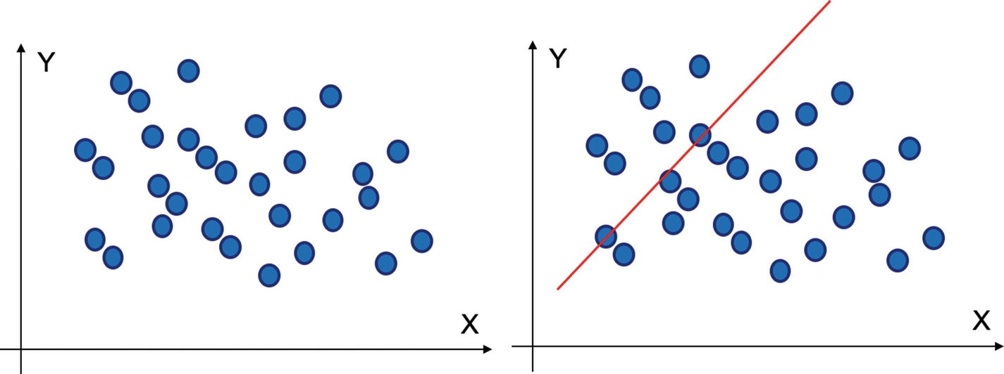
- 1.
Our model equation takes a serious hit in the case of outliers, as visible in Figure 5-5. In the presence of outliers, the regression equation tries to fit them too and hence the actual equation will not be the best one.

The impact of outliers on the regression equation makes it biased
- 2.
Outliers bias the estimates for the model and increase the error variance.
- 3.
If a statistical test is to be performed, its power and impact take a serious hit.
- 4.
Overall, from the data analysis, we cannot trust coefficients of the model and hence all the insights from the model will be erroneous.
Outlier Value of Temperature May Not Necessarily Be Bad and Hence Outliers Should Be Treated with Caution
- |

Hence, we should be cautious while we treat outliers. Blanket removal of outliers is not recommended!
- 1.
Recall we discussed normal distribution in Chapter 1. If a value lies beyond the 5th percentile and 95th percentile OR 1st percentile and 99th percentile we may consider it as an outlier.
- 2.
A value which is beyond –1.5 × IQR and +1.5 × IQR can be considered as an outlier. Here IQR is interquartile range and is given by (value at 75th percentile) – (value at 25th percentile).
- 3.
Values beyond one or two or three standard deviations from the mean can be termed as outliers.
- 4.
Business logic can also help in determining any unusual value to detect outliers.
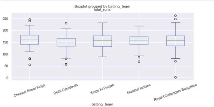
- 5.
We can visualize outliers by means of a box-plot or box-whiskers diagram. We have created box-plots in earlier chapters and will be revisiting in the next section.
- 1.
Delete the outliers completely. This is to be done after confirming that outliers can be deleted.
- 2.
Cap the outliers. For example, if we decide that anything beyond 5th percentile and 95th percentile is outlier, then anything beyond those values will be capped at 5th percentile and 95th percentile, respectively.
- 3.
Replace the outliers with mean, median, or mode. The approach is similar to the one we discussed for missing value treatment we discussed in the last section.
- 4.
Sometimes, taking a natural log of the variable reduces the impact of outliers. But again a cautious approach should be taken if we decide to take a natural log as it changes the actual values.
Outliers pose a big challenge to our datasets. They skew the insights we have generated from the data. Our coefficients are skewed and the model gets biased, and hence we should be cognizant of their impact. At the same time, we cannot ignore the relation of the business world with outliers and gauge if the observation is a serious outlier.
Apart from the issues discussed previously, there are quite a few other challenges faced in real-world datasets. We discuss some of these challenges in the next section.
Other Common Problems in the Dataset
We have seen the most common issues we face with our datasets. And we studied how to detect those defects and how to fix them. But real-world datasets are really messy and unclean, and there are many other factors which make a proper analysis fruitful.
- 1.
Correlated variables: if the independent variables are correlated with each other, it does not allow us to measure the true capability of our model. It also does not generate correct insights about the predictive power of the independent variables. The best way to understand collinearity is by generating a correlation matrix. This will guide us towards the correlated variables. We should test multiple combinations of input variables and if there is no significant drop in accuracy or pseudo R2, we can drop one of the correlated variables. We have dealt with the problem of correlated variables in the previous chapters of the book.
- 2.Sometimes there is only one value present in the entire column. For example, in Table 5-11.Table 5-11
Temperature Has Only One Value and Hence Is Not Adding Any Information
-
Temperature has a constant value of 1. It will not offer any significant information to our model and hence it is our best interest to drop this variable.
- 3.
An extension to the preceding point can be, if a particular variable has only two or three unique values. For example, consider a case when the preceding dataset has 100,000 rows. If the unique values of temperature are only 100 and 101, then it too will not be of much benefit. However, it might be as good as a categorical variable.
Such variables will not add anything to the model and will unnecessarily reduce pseudo R2.
- 4.
Another way to detect such variables is to check their variance. The variance of the variables discussed in Point 1 will be 0 and for the ones discussed in Point 2 will be quite low. So, we can check the variance of a variable, and if it is below a certain threshold, we can examine those variables further.
- 5.
It is also imperative that we always ensure that the issues discussed during the data discovery phase in the previous section are tackled. If not, we will have to deal with them now and clean them!
- 1.
Standardization or z-score: here we transform the variable as shown the formula.

This is the most popular technique. It makes the mean as 0 and standard deviation as 1
- 2.
Normalization is done to scale the variables between 0 and 1 retaining their proportional range to each other. The objective is to have each data point same scale so that each variable is equally important, as shown in Equation 5-1.
 (Equation 5-1)
 - 3.
Min-max normalization is used to scale the data to a range of [0,1]; it means the maximum value gets transformed to 1 while the minimum gets a value of 0. All the other values in between get a decimal value between 0 and 1, as shown in Equation 5-2.
 (Equation 5-2)
Since Min-max normalization scales data between 0 and 1, it does not perform very well in case there are outliers present in the dataset. For example, if the data has 100 observations, 99 observations have values between 0 and 10 while 1 value is 50. Since 50 will now be assigned “1,” this will skew the entire normalized dataset.
- 4.
Log transformation of variables is done to change the shape of the distribution, particularly for tackling skewness in the dataset.
- 5.
Binning is used to reduce the numeric values to categorize them. For example, age can be categorized as young, middle, and old.
This data-cleaning step is not an easy task. It is really a tedious, iterative process. It does test patience and requires business acumen, dataset understanding, coding skills, and common sense. On this step, however, rests the analysis we do and the quality of the ML model we want to build.
Now, we have reached a stage where we have the dataset with us. It might be cleaned to a certain extent if not 100% clean.
We can now proceed to the EDA stage, which is the next topic.
Step 4: EDA
EDA is one of the most important steps in the ML model-building process. We examine all the variables and understand their patterns, interdependencies, relationships, and trends. Only during the EDA phase will we come to know how the data is expected to behave. We uncover insights and recommendations from the data in this stage. A strong visualization complements the complete EDA.
EDA is the key to success. Sometimes proper EDA might solve the business case.
There is a thin line between EDA and the data-cleaning phase. Apparently, the steps overlap between data preparation, feature engineering, EDA, and data-cleaning phases.
EDA has two main heads: univariate analysis and bivariate analysis. Univariate, as the name suggests, is for an individual variable. Bivariate is used for understanding the relationship between two variables.
We will now complete a detailed case using Python. You can follow these steps for EDA. For the sake of brevity, we are not pasting all the results here. The dataset and code are available at the Github link at https://github.com/Apress/supervised-learning-w-python/tree/master/Chapter%205.


We have developed correlation metrics earlier in the book. Apart from these, there are multiple ways to perform the EDA. Scatter plots, crosstabs, and so on serve as a good tool.
EDA serves as the foundation of a robust ML model. Unfortunately, EDA is often neglected or less time is spent on it. It is a dangerous approach and can lead to challenges in the model at a later stage. EDA allows us to measure the spread of all the variables, understand their trends and patterns, uncover mutual relationships, and give a direction to the analysis. Most of the time, variables which are coming as important during EDA will be found significant by the ML model too. Remember, the time spent on EDA is crucial for the success of the project. It is a useful resource to engage the stakeholders and get their attention, as most of the insights are quite interesting. Visualization makes the insights even more appealing. Moreover, an audience which is not from an ML or statistical background will be able to relate to EDA better than to an ML model. Hence, it is prudent to perform a robust EDA of the data.
Now it is time to discuss the ML model-building stage in the next section.
Step 5: ML Model Building
Now we will be discussing the process we follow during the ML model development phase. Once the EDA has been completed, we now have a broad understanding of our dataset. We somewhat are clear on a lot of trends and correlations present in our dataset. And now we have to proceed to the actual model creation phase.
We are aware of the steps we follow during the actual model building. We have solved a number of case studies in the previous chapters. But there are a few points which we should be cognizant of while we proceed with model building. These cater to the common issues we face or the usual mistakes which are made. We will be discussing them in this section.
We will be starting with the training and testing split of the data.
Train/Test Split of Data
We understand that the model is trained on the training data and the accuracy is tested on the testing/validation dataset. The raw data is split into train/test or train/test/validate. There are multiple ratios which are used. We can use 70:30 or 80:20 for train/test splitting. We can use 60:20:20 or 80:10:10 for train/test/validate split, respectively.
- 1.
The training data should be representative of the business problem. For example, if we are working on a prepaid customer group for a telecom operator it should be only for prepaid customers and not for postpaid customers, though this would have been checked during the data discovery phase.
- 2.
There should not be any bias while sampling the training or testing datasets. Sometimes, during the creation of training or testing data, a bias is introduced based on time or product. This has to be avoided since the training done will not be correct. The output model will be generating incorrect predictions on the unseen data.
- 3.
The validation dataset should not be exposed to the algorithm during the training phase. If we have divided the data into train, test, and validation datasets, then during the training phase we will check the model’s accuracy on the train and test datasets. The validation dataset will be used only once and in the final stage once we want to check the robustness.
- 4.
All the treatments like outliers, null values, and so on should be applied to the training data only and not to the testing dataset or the validation dataset.
- 5.The target variable defines the problem and holds the key to the solution. For example, a retailer wishes to build a model to predict the customers who are going to churn. There are two aspects to be considered while creating the dataset:
- a.The definition of target variable or rather the label for it will decide the design of the dataset. For example, in Table 5-12 if the target variable is “Churn” then the model will predict the propensity to churn from the system. If it is “Not Churn,” it will mean the propensity to stay and not churn from the system.Table 5-12
Definition of Target Variable Changes the Entire Business Problem and Hence the Model
-

- b.
The duration we are interested in predicting the event. For example, customers who are going to churn in the next 60 days are going to be different from the ones who will churn in 90 days, as shown in Figure 5-6.
- a.

The customer datasets are subsets of each other. For example, customers who are going to churn in 30 days will be a subset of the ones who are going to churn in 90 days.
Creation of training and testing data is the most crucial step before we do the actual modeling. If there is any kind of bias or incompleteness in the datasets created, then the output ML model will be biased.
Once we have secured the training and testing dataset, we move to the next step of model building.
Model Building and Iterations

The arrangement of various algorithms with respect to accuracy and interpretability
Generally, we start with a base algorithm like linear regression or logistic regression or decision tree. This sets the basic benchmark for us for the other algorithms to break.
Then we proceed to train the algorithm with other classification algorithms. There is a tradeoff which always exists, in terms of accuracy, speed of training, prediction, robustness, and ease of comprehension. It also depends on the nature of the variables; for example, k-nearest neighbor requires numeric variables as it needs to calculate the distance between various data points. One-hot encoding will be required to convert categorical variables to the respective numeric values.
- 1.
Create the base version of the algorithm using logistic regression or decision tree.
- 2.
Measure the performance on a training dataset.
- 3.
Iterate to improve the training performance of the model. During iterations, we try a combination of addition or removal of variables, changing the hyperparameters, and so on.
- 4.
Measure the performance on a testing dataset.
- 5.
Compare the training and testing performance; the model should not be overfitting (more on this in the next section).
- 6.
Test with other algorithms like random forest or SVM and perform the same level of iterations for them.
- 7.
Choose the best model based on the training and testing accuracy.
- 8.
Measure the performance on the validation dataset.
- 9.
Measure the performance on out-of-time dataset.

At the end of this step, we would have accuracies of various algorithms with us. We are discussing the best practices for accuracy measurement now.
Accuracy Measurement and Validation
Comparing the Performance Measurement Parameters for All the Algorithms to Choose the Best One
|

Then we can take a decision to choose the best algorithm. The decision to choose the algorithm will also depend on parameters like time taken to train, time taken to make a prediction, ease of deployment, ease of refresh, and so on.
Along with the accuracy measurement, we also check time taken to prediction and the stability of the model. If the model is intended for real-time prediction, then time taken to predict becomes a crucial KPI.
At the same time, we have to validate the model too. Validation of the model is one of the most crucial steps. It checks how the model is performing on the new and unseen dataset. And that is the main objective of our model: to predict well on new and unseen datasets!
It is always a good practice to test the model’s performance on an out-of-time dataset. For example, if the model is trained on a Jan 2017 to Dec 2018 dataset, we should check the performance on out-of-time data like Jan 2019–Apr 2019. This ensures that the model is able to perform on the dataset which is unseen and not a part of the training one. We will now study the impact of threshold on the algorithm and how can we optimize in the next section.
Finding the Best Threshold for Classification Algorithms
There is one more important concept of the most optimum threshold, which is useful for classification algorithms. Threshold refers to the probability score above which an observation will belong to a certain class. It plays a significant role in measuring the performance of the model.
For example, consider we are building a prediction model which will predict if a customer will churn or not. Let’s assume that the threshold set for the classification is 0.5. Hence, if the model generates a score of 0.5 or above for a customer, the customer is predicted to churn; otherwise not. It means a customer with a probability score of 0.58 will be classified as a “predicted to churn.” But if the threshold is changed to 0.6, then the same customer will be classified as a “non-churner.” This is the impact of setting the threshold.
The default threshold is set at 0.5, but this is generally unsuitable for unbalanced datasets. Optimizing the threshold is an important task, as it can seriously impact the final results.
We can optimize the threshold using the ROC curve. The best threshold is where True Positive Rate and (1- False Positive Rate) overlap with each other. This approach maximizes the True Positive Rate while minimizing the False Positive Rate. However, it is recommended to test the performance of the model at different values of threshold to determine the best value. The best threshold will also depend on the business problem we are trying to solve.
There is one common problem we encounter during the model development phase: overfitting and underfitting, which we will discussing now.
Overfitting vs. Underfitting Problem

Bias-variance tradoff. Note that the optimal model complexity is the sweet spot where both bias and variance are balanced
Underfitting where a very simple model has been created

Overfitting where a very complex model has been created
Underfitting can be tackled by increasing the complexity of the model. Underfitting means that we have chosen a very simplistic solution for our ML approach while the problem at hand requires a higher degree of complexity. We can easily identify a model which is underfitting. The model’s training accuracy will not be good and hence we can conclude the model is not even able to perform well on the training data. To tackle underfitting, we can train a deeper tree, or instead of fitting a linear equation, we can fit a nonlinear equation. Using an advanced algorithm like SVM might give improved results.
Sometimes there is no pattern in the data. Even using the most complex ML algorithm will not lead to good results. In such a case, a very strong EDA might help.
- 1.
Maybe the easiest approach is to train with more data. But this might not always work if the new dataset is messy or if the new dataset is similar to the old one without adding additional information.
- 2.
k-fold cross-validation is a powerful method to combat overfitting. It allows us to tweak the respective hyperparameters and the test set will be totally unseen till the final selection has to be made.
The k-fold validation technique is depicted in Figure 5-11. It is a very simple method to implement and understand. In this technique, we iteratively divide the data into training and testing “folds.”
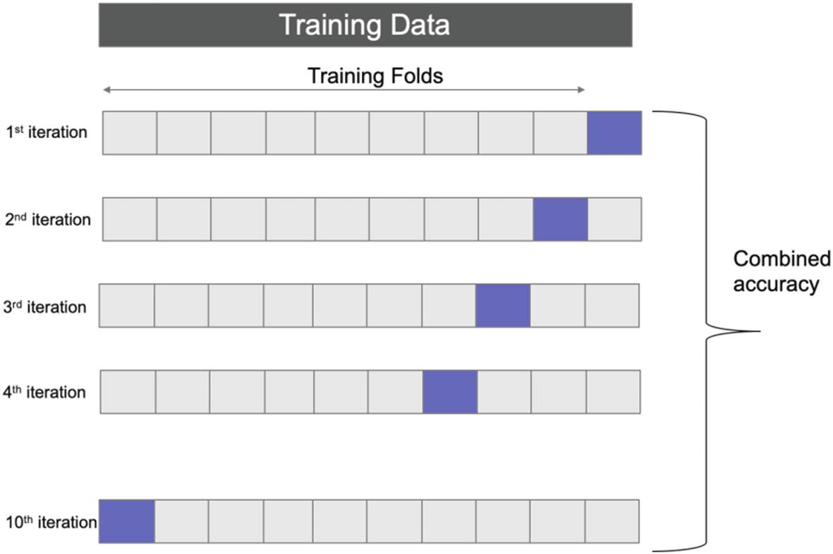
k-fold cross-validation is a fantastic technique to tackle overfitting
- 1.
We shuffle the dataset randomly and then split into k groups.
- 2.
For each of the groups, we take a test set. The remaining serve as a training set.
- 3.
The ML model is fit for each group by training on the training set and testing on the test set (also referred as holdout set).
- 4.
The final accuracy is the summary of all the accuracies.
It means that each data point gets a chance to be a part of both the testing and the training dataset. Each observation remains a part of a group and stays in the group during the entire cycle of the experiment. Hence, each observation is used for testing once and for training (k–1) times.
The Python implementation of the k-fold validation code is checked in at the Github repo.
- 3.
Ensemble methods like random forest combat overfitting easily as compared to decision trees.
- 4.
Regularization is one of the techniques used to combat overfitting. This technique makes the model coefficients shrink to zero or nearly zero. The idea is that the model will be penalized if a greater number of variables are added to the equation.
There are two types of regularization methods: Lasso (L1) regression and Ridge (L2) regression. Equation 5-3 may be recalled from earlier chapters.
 (Equation 5-3)
At the same time, we have a loss function which has to be optimized to receive the best equation. That is the residual sum of squares (RSS).
In Ridge regression, a shrinkage quantity is added to the RSS, as shown in Equation 5-4.
So, the modified (Equation 5-4)
Here λ is the tuning parameter which will decide how much we want to penalize the model. If λ is zero, it will have no effect, but when it becomes large, the coefficients will start approaching zero.
In Lasso regression, a shrinkage quantity is added to the RSS similar to Ridge but with a change. Instead of squares, an absolute value is taken, as shown in Equation 5-5.
So the modified (Equation 5-5)
Between the two models, ridge regression impacts the interpretability of the model. It can shrink the coefficients of very important variables to close to zero. But they will never be zero, hence the model will always contain all the variables. Whereas in lasso some parameters can be exactly zero, making this method also help in variable selection and creating sparse models.
- 5.Decision trees generally overfit. We can combat overfitting in decision tree using these two methods:
- a.
We can tune the hyperparameters and set constraints on the growth of the tree: parameters like maximum depth, maximum number of samples required, maximum features for split, maximum number of terminal nodes, and so on.
- b.
The second method is pruning. Pruning is opposite to building a tree. The basic idea is that a very large tree will be too complex and will not be able to generalize well, which can lead to overfitting. Recall that in Chapter 4 we developed code using pruning in decision trees.
Decision tree follows a greedy approach and hence the decision is taken only on the basis of the current state and not dependent on the future expected states. And such an approach eventually leads to overfitting. Pruning helps us in tackling it. In decision tree pruning, we- i.
Make the tree grow to the maximum possible depth.
- ii.
Then start at the bottom and start removing the terminal nodes which do not provide any benefit as compared to the top.
- i.
- a.
Note that the goal of the ML solution is to make predictions for the unseen datasets. The model is trained on historical training data so that it can understand the patterns in the training data and then use the intelligence to make predictions for the new and unseen data. Hence, it is imperative we gauge the performance of the model on testing and validation datasets. If a model which is overfitting is chosen, it will fail to work on the new data points, and hence the business reason to create the ML model will be lost.
The model selection is one of the most crucial yet confusing steps. Many times, we are prone to choose a more complex or advanced algorithm as compared to simpler ones. However, if a simpler logistic regression algorithm and advanced SVM are giving similar levels of accuracy, we should defer to the simpler one. Simpler models are easier to comprehend, more flexible to ever-changing business requirements, straightforward to deploy, and painless to maintain and refresh in the future. Once we have made a choice of the final algorithm which we want to deploy in the production environment, it becomes really difficult to replace the chosen one!
The next step is to present the model and insights to the key stakeholders to get their suggestions.
Key Stakeholder Discussion and Iterations
It is a good practice to keep in close touch with the key business stakeholders. Sometimes, there are some iterations to be done after the discussion with the key stakeholders. They can add their inputs using business acumen and understanding.
Presenting the Final Model
The ML model is ready. We have had initial rounds of discussions with the key stakeholders. Now is the time when the model will be presented to the wider audience to take their feedback and comments.
We have to remember that an ML model is to be consumed by multiple functions of the business. Hence, it is imperative that all the functions are aligned on the insights.
Congratulations! You have a functional, validated, tested, and (at least partially) approved model. It is then presented to all the stakeholders and team for a detailed discussion. And if everything goes well, the model is ready to be deployed in production.
Step 6: Deployment of the Model
We have understood all the stages in model development so far. The ML model is trained on historical data. It has generated a series of insights and a compiled version of the model. It has to be used to make predictions on the new and unseen dataset. This model is ready to be put into the production environment, which is referred to as deployment. We will examine all the concepts in detail now.
ML is a different type of software as compared to traditional software engineering. For an ML model, several forces join hands to make it happen. It is imperative we discuss them now because they are the building blocks of a robust and useful solution.

Key elements of an ML solution which are the foundation of the solution
- 1.
Interdependency in an ML solution refers to the relationship between the various variables. If the values of one of the variables change, it does make an impact on the values of other variables. Hence, the variables are interdependent on each other. At the same time, the ML model sometimes is quite “touchy” to even a small change in the values of the data points.
- 2.
Data lies at the heart of the model. Data powers the model; data is the raw material and is the source of everything. Some data points are however very unstable and are always in flux. It is hence imperative that we track such data changes while we are designing the system. Model and data work in tandem with each other.
- 3.
Errors happen all the time. There are many things we plan for a deployment. We ensure that we are deploying the correct version of the algorithm. Generally, it is the one which has been trained on the latest dataset and which has been validated.
- 4.
Reproducibility is one of the required and expected but difficult traits for an ML model. It is particularly true for models which are trained on a dynamic dataset or for domains like medical devices or banks which are bound with protocols and rules. Imagine an image classification model is built to segregate good vs. bad products based on images in a medical devices industry. In a case like that, the organization will have to adhere to protocols and will be submitting a technical report to the regulatory authorities.
- 5.
Teamwork lies at the heart of the entire project. An ML model requires time and attention from a data engineer, data analyst, data scientist, functional consultant, business consultant, stakeholder, dev ops engineer, and so on. For the deployment too, we need guidance and support from some of these functions.
- 6.
Business stakeholder and sponsors are the key to a successful ML solution. They will be guiding how the solution can be consumed and will be used to resolve the business problem.
Deployment is not an easy task; it requires time, teamwork, and multiple skills to handle.
- 1.
We have to check if the ML model is going to work in real time or in a batch prediction mode. For example, checking if an incoming transaction is fraudulent or not is an example of a real-time check. If we are predicting if a customer will default or not, that’s not a real-time system but a batch prediction mode and we have the luxury to make a prediction maybe even the next day.
- 2.
The size of the data we are going to deal with is a big question to be answered. And so it is important to know the size of the incoming requests. For example, if an online transaction system expects 10 transactions per second as compared to a second system which expects 1000 transactions, load management and speed of decision will make a lot of difference.
- 3.
We also make sure to check the performance of the model in terms of time it takes to predict, stability, what the memory requirements are, and how is it producing the final outputs.
- 4.Then we also decide if the model requires on-off training or real-time training.
- a.
On-off training is where we have trained the model of historical data and we can put it in production till its performance decays. Then we will be refreshing the model.
- b.
Real-time training allows the ML model to be trained on a real-time dataset and then get retrained. It allows the ML model to always cater to the new dataset.
- a.
- 5.
The amount of automation we expect in the ML model is to be decided. This will help us to plan the manual steps better.
- 1.It all starts with having a database. The database can be in the cloud or a traditional server. It contains all the tables and sources from which the model is going to consume the incoming data as shown in Figure 5-13. Sometimes, a separate framework feeds the data to the model.
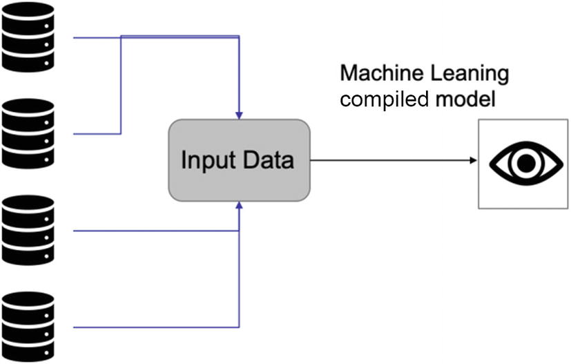 Figure 5-13
An ML model can take input data from multiple sources
- 2.
In case a variable is not a raw variable but a derived one, the same should have been taken care of in the creation of the data source for the data. For example, consider for a retailer, the incoming raw data is customer transactions details of the day. We built a model to predict the customer churn, and one of the significant variables is the customer’s average transaction value (total revenue/number of transactions); then this variable will be a part of the data provider tables.
- 3.
This incoming data is unseen and new to the ML model. The data contains the data in the format expected by the compiled model. If the data is not in the format expected, then there will be a runtime error. Hence, it is imperative that the input data is thoroughly checked. In case we have an image classification model using a neural network, we should check that the dimensions of the input image are the same as expected by the network. Similarly, for structured data it should be checked that the input data is as expected and is checked including the names and type of the variables (integer, string, Boolean, data frame, etc.).
- 4.The compiled model is stored as a serialized object like .pkl for Python, .R file for R, .mat for MATLAB, .h5, and so on. This is the compiled object which is used to make the predictions. There are a few formats which can be used:
- a.
Pickle format is used for Python. The object is a streamed object which can be loaded and shared across. It can be used at a later point too.
- b.
ONNX (Open Neural Network Exchange Format) allows storing of predictive models. Similarly, PMML (Predictive Model Markup languages) is another format which is used.
- a.
- 5.
The objective of the model, the nature of predictions to be made, the volume of the incoming data, real-time prediction or on-off prediction, and so on, allow us to design a good architecture for our problem.
- 6.When it comes to the deployment of the model, there are multiple options available to us. We can deploy the model as follows:
- a.
Web service : ML models can be deployed as a web service. It is a good approach since multiple interfaces like web, mobile, and desktop are handled. We can set up an API wrapper and deploy the model as a web service. The API wrapper is responsible for the prediction on the unseen data.
Using a web service approach, the web service can take an input data and convert into a dataset or data frame as expected by the model. Then, it can make a prediction using the dataset (either continuous variable or a classification variable) and return the respective value.
Consider this. A retailer sells specialized products online. A lot of the business comes from repeat customers. Now a new product is launched by the retailer. And the business wants to target the existing customer base.
So, we want to deploy an ML model which predicts if the customer will buy a newly launched product based on the last transactions by the customer. We have depicted the entire process in Figure 5-14. Figure 5-14
Web service–based deployment process
We should note that we already have historical information on the customer’s past behavior. Since there is a need to make a prediction on a new set of information, the information has to be merged and then shared with the prediction service.
As a first step, the website or the app initializes and makes a request to the information module. The information module consists of information about customer’s historical transactions, and so on. It returns this information about the customer to the web application. The web app initializes the customer’s profile locally and stores this information locally. Similarly, the new chain of events or the trigger which is happening at the web or in the app is also obtained. These data points (old customer details and new data values) are shared with a function or a wrapper function which updates the information received based on the new data points. This updated information is then shared with the prediction web service to generate the prediction and receive the values back.
In this approach, we can use AWS Lambda functions, Google Cloud functions, or Microsoft Azure functions. Or we can use containers like Docker and use it to deploy a flask or Django application.
- a.
- b.Integrated with the database: Perhaps this approach is generally used. As shown in Figure 5-15, this approach is easier than a web service–based one but is possible for smaller databases.
 Figure 5-15
Integration with database to deploy the model
In this approach, the moment a new transaction takes place an event is generated. This event creates a trigger. This trigger shares the information to the customer table where the data is updated, and the updated information is shared with the event trigger. Then the prediction model is run, and a prediction score is generated to predict if the customer will make a purchase of the newly launched product. And finally, the customer data is again updated based on the prediction made.
This is a simpler approach. We can use databases like MSSQL, PostGres, and so on.
We can also deploy the model into a native app or as a web application. The predictive ML model can run externally as a local service. It is not heavily used. Once the model is deployed, the predictions have to be consumed by the system.
- 7.The next step to ponder over is consumptions of the predictions done by the ML model.
- a.
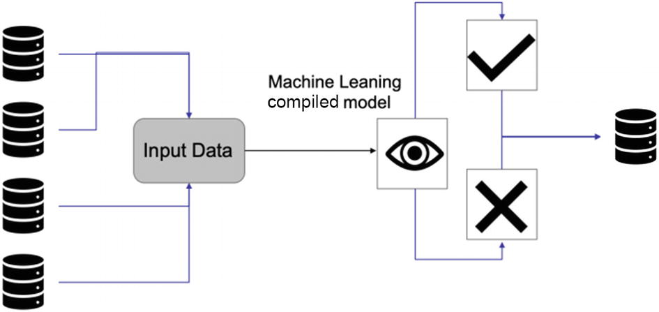
If the model is making a real-time prediction as shown in Figure 5-16, then the model can return a signal like pass/fail or yes/no. The model can also return a probability score, which can then be handled by the incoming request.
- a.

Real-time prediction system takes seconds or milliseconds to make a prediction
- b.
If the model is not a real-time model, then it is possible that the model is generating probability scores which are to be saved into a separate table in the database. It is referred to as batch prediction, as shown in Figure 5-17. Hence, the model-generated scores have to be written back to the database. It is not necessary to write back the predictions. We can have the predictions written in a .csv or .txt file, which can then be uploaded to the database. Generally, the predictions are accompanied by all the details of the raw incoming data for which the respective prediction has been made.
The predictions made can be continuous in case of a regression problem or can be a probability score/class for a classification problem. Depending on the predictions, we can make configurations accordingly.
Batch prediction is saved to a database
- 8.We can use any cloud platform which allows us to create, train, and deploy the model too. Some of the most common options available are
- a.
AWS SageMaker
- b.
Google Cloud AI platform
- c.
Azure Machine Learning Studio, which is a part of Azure Machine Learning service
- d.
IBM Watson Studio
- e.
Salesforce Einstein
- f.
MATLAB offered by MathWorks
- g.
RapidMiner offers RapidMiner AI Cloud
- h.
TensorFlow Research Cloud
- a.
Congratulations! The model is deployed in the production and is making predictions on real and unseen dataset. Exciting, right?
Step 7: Documentation
Our model is deployed now we have to ensure that all the codes are cleaned, checked in, and properly documented. Github can be used for version control.
Documentation of the model is also dependent on the organization and domain of use. In regulated industries it is quite imperative that all the details are properly documented.
Step 8: Model Refresh and Maintenance
We have understood all the stages in model development and deployment now. But once a model is put into production, it needs constant monitoring. We have to ensure that the model is performing always at a desired level of accuracy measurements. To achieve this, it is advised to have a dashboard or a monitoring system to gauge the performance of the model regularly. In case of non-availability of such a system, a monthly or quarterly checkup of the model can be done.

ML model refresh and maintenance process
Once the model is deployed, we can do a monthly random check of the model. If the performance is not good, the model requires refresh. It is imperative that even though the model might not be deteriorating, it is still a good practice to refresh the model on the new data points which are constantly created and saved.
With this, we have completed all the steps to design an ML system, how to develop it from scratch, and how to deploy and maintain it. It is a long process which is quite tedious and requires teamwork.
With this, we are coming to the end of the last chapter and the book.
Summary
In this last chapter we studied a model’s life—from scratch to maintenance. There can be other methods and processes too, depending on the business domain and the use case at hand.
With this, we are coming to the end of the book. We started this book with an introduction to ML and its broad categories. In the next chapter, we discussed regression problems, and then we solved classification problems. This was followed by much more advanced algorithms like SVM and neural networks. In this final chapter, we culminated the knowledge and created the end-to-end model development process. The codes in Python and the case studies complemented the understanding.
Data is the new oil, new electricity, new power, and new currency. The field is rapidly increasing and making its impact felt across the globe. With such a rapid enhancement, the sector has opened up new job opportunities and created new job titles. Data analysts, data engineers, data scientists, visualization experts, ML engineers—they did not exist a decade back. Now, there is a huge demand of such professionals. But there is dearth of professionals who fulfill the rigorous criteria for these job descriptions. The need of the hour is to have data artists who can marry business objectives with analytical problems and envision solutions to solve the dynamic business problems.
Data is impacting all the business, operations, decisions, and policies. More and more sophisticated systems are being created everyday. Data and its power are immense: we can see examples of self-driving cars, chatbots, fraud detection systems, facial recognition solutions, object detection solutions, and so on. We are able to generate rapid insights, scale the solutions, visualize, and take decisions on the fly. The medical industry can create better drugs, the banking and financial sectors can mitigate risks, telecom operators can offer better and more stable network coverages, and the retail sector can provide better prices and serve the customers better. The use cases are immense and still being explored.
But the onus lies on us on how to harness this power of data. We can put it to use for the benefit of mankind or for destroying it. We can use ML and AI for spreading love or hatred—it is our choice. And like the cliché goes—with great power comes great responsibility!
Question 1: What is overfitting and how can we tackle it?
Question 2: What are the various options available to deploy the model?
Question 3: What are the types of variable transformations available?
Question 4: What is the difference between L1 and L2 regularization?
Question 5: Solve the exercises we did in previous chapters and compare the accuracies after treating missing values and correlated variables.
Question 6: What are the various steps in EDA?
Question 7: Download the NFL dataset from the following link and treat for the missing values: https://www.kaggle.com/maxhorowitz/nflplaybyplay2009to2016.
Question 8: How can we define an effective business problem?