
It is a capital mistake to theorize before one has data. Insensibly one begins to twist facts to suit theories, instead of theories to suit facts.
—Sherlock Holmes, “A Study in Scarlet” (1877)
Readability since the wrong data structures can make the code more complex than what actually required.
- Better design because they are strictly related to project’s requirements:
How data can be better organized?
How to improve performances?
Are there any memory constraints?
Fun: yes, you’ll have a lot of fun with them.
In this chapter, we will introduce common data structures and how to evaluate them in the overall grand scheme of designing clean code.
Introduction to Data Structures
Time Complexity
Data Structure | Access | Insert | Delete | Search |
|---|---|---|---|---|
Array | O(1) | O(n) | O(n) | O(n) |
Linked list | O(n) | O(1) | O(1) | O(n) |
Doubly linked list | O(n) | O(1) | O(1) | O(n) |
Queue | O(n) | O(1) | O(1) | O(n) |
Stack | O(n) | O(1) | O(1) | O(n) |
Hash map | Constant (avg) | O(1) | O(1) | O(1) |
Binary search tree | O(n log n) | O(n log n) | O(n log n) | O(n log n) |
Taking into account the performances of a given data structure should not be an afterthought. And it matches well the good-design way of proceeding. The more suitable the data structures, the more optimized, effective, and efficient the design is.
Asymptotic analysis (as shown in Table 3-1) allows to express time performances in the context of the size of the data (i.e., the number of elements). In short, if an operation always takes the “same” amount of time (i.e., not dependent on the size of the data), we say that it has constant time and we refer to it as O(1). If an operation scales logarithmically with the data size, we refer to it as O(log n). If an operation scales linearly with the data size, we say that it runs in linear time and we refer to it as O(n). Operations can also scale in polynomial (e.g., O(n2)) and exponential (e.g., O(2n)) time. Always try to understand if and how polynomial and exponential operations can be optimized.
Data size
Does the data changes and how often?
Are search and sorting operation frequent?
When reasoning around data size, do not focus only on the problem at hand. Try to look at possible future cases and how data might possibly scale over time. This would help not only in considering data in the context at hand but also spotting any limiting or better options in terms of runtime.
A very well-known principle, which can be applied to data structure as well, is the Pareto principle, also known as the 80/20 principle. This principle states that 20% of causes generate 80% of the results.
As you will read in the rest of the chapter, every data structure comes not only with a general context that might suit them better. They also come with different runtimes for common operation (e.g., adding and deleting elements). To pick and validate data structure, one of the approaches you can explore is to think about the 80% of operations that you need to perform on a given set of data and evaluate which data structure would be the most performant (runtime) data structure to use in such context.
Consider a scenario where 80% of operations are given by adding and searching elements in a data structure. As from Table 3-1, you can start confronting time complexity. Would it be optimal to use a linked list with O(n) search? Definitely not. By using HashMaps, you could have a better running time since by design HashMaps suit really good searching operations with a constant average runtime.
Let’s go through the pros and cons of each data structure.
Array
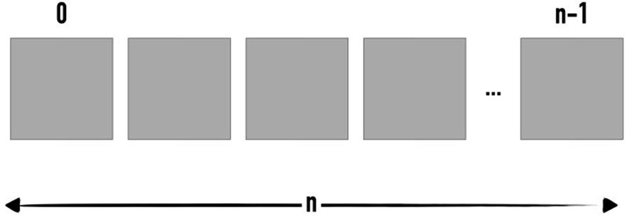
Array
Each box in Figure 3-1 represents an element within the array, each of which with a relative position within the array. Position counting always starts at 0.
Basic arrays are fixed in size, which is the size declared during initialization. They support only a single type (e.g., all integers).
where the first parameter ‘i’ specifies the typecode, which in the specific case refers to signed integers of 2 bytes. The second parameter provides initializers for the given array.
As you might have noted already from the first snippet of code, the array requires the import of the standard module “array.” This is because Python does not natively support arrays. Other libraries, including NumPy, also provide their own implementation of arrays. However, it is pretty common to use Python lists in day-to-day code instead of arrays due to their flexibility.
They come with several pros and cons.
They are fairly easy to use and—as shown in Table 3-1—they provide direct access by means of indexes, and the entire list of elements can be accessed linearly in O(n), where n is the number of elements into the list.
However, inserting and deleting items from the list are more computationally expensive due to shifting operation required to perform these operations. As a worst-case scenario, to better understand why it happens, consider deleting the first element of the list which is at index = 0. This operation creates an empty spot; thus all the items from index = 1 need to be shifted one position backward. This gives us a complexity of O(n). Analogous considerations are for insertion.
Linked List

Linked list
Compared to arrays, add and remove operations are easier because no shifting is required. Removing an item from the list can be performed by changing the pointer of the element prior to the one that needs to be removed. Time complexity is still O(n) in the worst case. Indeed, in order to find the item that needs to be removed, it is required to navigate the entire list up to the searched element. The worst case happens when the removal needs to be done on the last element into the list. Often linked lists serve well as underlying implementation of other data structures including stacks and queues.
Doubly Linked List

Doubly linked list
Adding is slightly more complex than the previous type due to more pointers to be updated. Add and remove operations still take O(n) due to sequential access needed to locate the right node. In a figurative way, think about this doubly linked list as the navigation bar into your Google search. You have the current page (the node) and two links (pointers) to the previous and following page. Another example is the command history. Suppose you are editing a document. Each action you perform on the text (type text, erase, add image) can be considered a node which is added to the list. If you click the undo button, the list would move to the previous version of changes. Clicking redo would push you forward one action into the list.
Stack

Stack
- 1.
Top( ): Which returns the element on top of the stack
- 2.
Pop( ): Which removes the element on top and returns it
- 3.
Put( ): Which adds a new element on top of the stack
It suits well certain categories of problems including pattern validation (e.g., well-parenthesized expressions) as well as general parsing problems due to the LIFO policy.
Queue

Queue
- 1.
Peak( ): Which returns the first element in the queue
- 2.
Remove( ): Which removes the first element and returns it
- 3.
Add( ): Which adds a new element at the end of the queue
Queues are commonly used in concurrent scenarios, where several tasks need to be processed or for messaging management. Generally, queues can be used when order preservation is needed, hence problems that benefit from a FIFO approach. As an example, queues see common usage in cases where asynchronous messages are sent to a single point from different sources to a single processing point. In this scenario, queues are used for synchronization purposes. A real-world case of queue utilization is a printer, both shared (e.g., office printer) and personal. In both cases, multiple file can be sent simultaneously to the printer. However, the printer will queue them depending on arrival and will serve them in arrival time order (the first file to arrive is the first file to be printed).
Hash Map
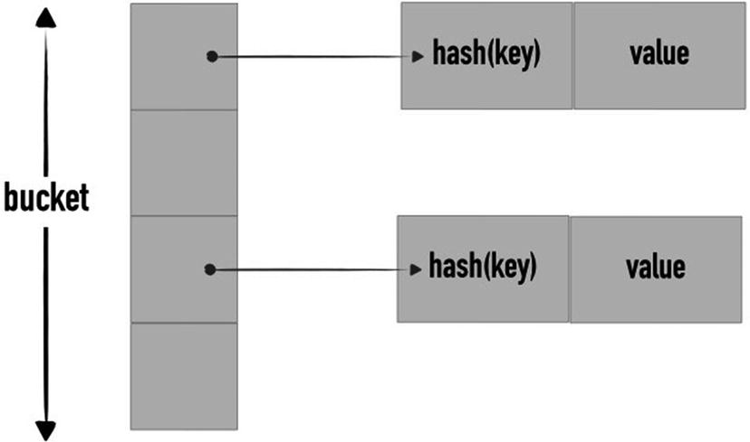
Hash map
As the name of this data structures expresses, keys are stored in locations (also referred to as slots) based on their hash code. Upon insertion, a hash function is applied to the key, producing the hash code. Hash functions have to map the same key into the same hash code. However, it might also happen that two different keys correspond to the same hash code, hence resulting in a collision. A good hash function is meant to minimize collisions.
The runtime strictly depends on the strength of the hash function to uniformly spread objects across the bucket (generally represented as an array of keys).
Being pragmatic, hash maps have really good performances in real-world scenarios. An example of utilization is the phone agenda. Indeed, for every friend you have (keys), a phone number is attached to it (values). Every time you want to call a specific friend, you perform a search (lookout) of their name (key) and you get the relative phone number (value).
A common error that can happen when using this data structure is trying to modify the key element into the data structure. In such case, it might be that this data structure does not suit the problem you are trying to solve.
If instead of maintaining the key stable (i.e., Harry) and just updating the value of the entry (i.e., from Potter to a different surname), you are trying to imagine this data structure as being able to change the same entry into “James Potter,” you probably need to better think the problem and use a different data structure.
Binary Search Trees
Trees are other fairly commonly used data structures. A tree is a collection of elements, where each element has a value and an arbitrary number of pointers to other nodes (namely, children).
They are organized in a top-down fashion, meaning that pointers usually link nodes up to bottom and each node has a single pointer referencing to it. The first node in this data structure is called the root of the tree. Nodes with no children are the leaves of the tree. The leaves of the tree are also referred to as the frontier of the tree.
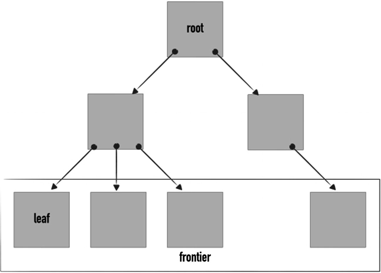
Tree
The left child’s value is less than or equal to the node’s value.
The right child’s value is greater than or equal to the node’s value.
The main benefit of this type of tree is that it enables a fast element search. Indeed, due to the ordering, each time half of the tree is excluded from the search (in the average case). As a consequence, binary search trees see sorting problems as one of their main applications.

Example of decision making using a tree representation
Every node in the example represents incrementally (top to bottom) alternatives at hand. By walking down the tree, indeed, you might decide that you are not going to the cinema, hence staying at home, and that you will watch TV, specifically Game of Thrones.
Options other than “Read this book” are an act of kindness from the author. Hope you are enjoying it so far!
Guidelines on Data Structures
Picking the appropriate data structure will become an innate capability as you keep developing code and as you expand your knowledge on the topic.
- 1.
Operations: Always start from the problem you are trying to solve. Which operations do you need to perform? Traversal? Search? Simple addition and removal? Do you need to be able to gather minimum or maximum of a given dataset?
- 2.
Ordering and sorting: Does your data scream for prioritization or any type of sorting of elements? FIFO? LIFO? Does the order need to be preserved? Does the data structure need to automatically handle data sorting?
- 3.
Uniqueness: Does your data require elements into the data structure to appear only once? There are data structures like sets that allow you to reflect uniqueness conditions.
- 4.
Relationship between elements: Does the data fit a hierarchical logical representation? Is the data more linear in nature? Do you need to logically group elements in a more complex way? This is the case, for example, where for each document, you want to be able to track for each word the number of occurrences of that word.
- 5.
Memory and time performances: As we seen in this chapter, every data structure has its own memory and time performances. The algorithms you are building on top of the data structure are heavily influenced by the performances of the operations you perform on data. The performance requirements you want to achieve are another key driver for exploring and filtering which data structure suits your needs.
- 6.
Complexity: If more than one data structure after all the filtering looks like a fit for purpose, opt for the most simple one.
By applying these criteria, you should be able to both better understand the problem and filter out data structures that do not suit your data and the context it is used in.
Design Use Case
Let’s analyze the example from the stack section: analyzing a sequence to ensure it is well parenthesized. In other words, we want to check that [()]()[()] is a correct way of using parenthesis, while [()]( is not. And we want to pick the right data structure that supports the problem we are trying to solve.
- 1.
We do not need complex operation: insertion and removal are all we need.
- 2.
It requires order preservation but no sorting capabilities.
- 3.
Elements are not unique.
- 4.
The problem is linear.
- 5.
The problem can be solved in linear time and memory.
And there is one data structure that suits the needs which is, as anticipated, the stack.
By being one of the simplest data structures available, we can also conclude that stacks are appropriate since we cannot simplify further given the requirements of the problem at hand.
Evaluation and Review
I love data structures. I promise that I will carefully consider them in my code reviews.
- 1.For every word in the array (left to right)
- a.
Initialize the relative element in the occurrences list with 1
- b.
Scan the remaining array
- c.
Every time the same word is found, update the relative entry into the occurrences list (i.e., increment of one)
- d.
Move to the next element (i.e., word) into the sentence array
- a.
Since for every word (n elements), we have to scan the remainder of the array (of size n), the time complexity is O(n2).
If we analyze the root problem a bit more carefully, we can quickly figure out that the main problem we are trying to solve is a search operation. This is our first red flag: arrays can be used but are not notoriously known for their search capabilities.
Ordering and sorting are not key elements in our problem: no matter what the order is, the result is not impacted by it. Arrays are okay in this regard.
The data is linear in nature, so arrays might fit.
Relationships between elements are our second red flag: we are using two separate data structures, but there is a strict relationship between each word in the sentence and relative counting.
Performance is another red flag; we don’t really like linear problems with polynomial time, don’t we?
Finally, we may assert that there is nothing more simple than arrays. And that would be true. This is a clear case where we might need to evaluate adding a tiny bit of complexity to get rid of the red flags. If well designed, the solution should not have been made that far.
And the king of optimized search able to express coupling relationship between elements is our dear hash map.
You can now implement changes accordingly. Interestingly enough, if you compare both solutions, the one using hash maps is also simpler and more readable.
The same approach can be applied to any programming interview you will face. More often than not, they do require implementing some sort of algorithm around data structure.
Summary
This chapter on data structures is not meant to be a data structure book. It aimed at doing a quick refresh on those you’ll end up using more often than not. At the end of the day, reviewing data structures is all about fit for purpose, not overcomplicating the code and considering the appropriate one in terms of memory and time performances.
- 1.
If you are trying to force the data structure to do operations that are not natively supported, it might not be the right one for your purpose.
- 2.
Even if the choice of data structure is surely related to the current problem you are trying to solve (e.g., data size), have a vision for possible growth and how it might impact the software.
- 3.
Use the 80/20 Pareto principle to help you choose the best data structure.
- 4.
Don’t opt for fancy data structures just for the sake of it. More complex data structure still requires some more memory management and processing. Always strive for a balance between scalability requirements and complexity. Simple is better, but it needs to get the job done.
In the next chapter, we will tackle code smells, what they are, and why they are bad for clean code and provide guidance on how to spot them in your software.
Further Reading
I love data structures. And amazing books are out there that dig deeper into various data structures and algorithms in general. At the top of my list is Introduction to Algorithms by Thomas H. Cormen (MIT Press, 2009). It is a must-read if you haven’t read it yet.
Code Review Checklist
- 1.
Are data structures appropriately used?
- 2.
Is the data structure appropriate based on the data size the code is dealing with?
- 3.
Are potential changes to data size considered and handled?
- 4.
Is the data structured forced to do operations not natively supported?
- 5.
Does the data structure support growth (i.e., scalability)?
- 6.
Does the data structure reflect the need for relationships between elements?
- 7.
Does the data structure optimally support the operations you need to perform on it?
- 8.
Is the choice of a specific data structure overcomplicating the code?
- 9.
Is the data structure chosen based on most frequent operations to be performed on data?
- 10.
Are you using stacks for problems that do not require FIFO?
- 11.
Are you using queues for problems that do not require LIFO?
- 12.
Does the data structure reflect any ordering on sorting requirements?
- 13.
From a logical perspective, is the code meant to update the key within a hash map? If so, rethink the problem and see if hash maps are the best data structure to deal with it.