By this point in the series, you should have a working robot. In previous chapters, I covered everything you need to know to install and program your robot. You’ve worked with motors, sensors, and communication between the Raspberry Pi and the Arduino. In Chapters 3 and 5, you learned to work with ultrasonic rangefinders using both Python and Arduino. The remainder of the book introduces new sensors, processing algorithms, and computer vision.
In this chapter, we work with infrared (IR) sensors. We look at different types of sensors. At the end of the chapter, we use a series of IR sensors to detect the edge of a surface and a line.
Infrared Sensors
An infrared (IR) sensor is any sensor that uses a light detector, tuned for the IR spectrum, to detect an IR signal. Generally, the IR sensor is paired with IR-emitting LED to provide the IR signal. The emissions from the LED are measured for intensity or presence.
Types of IR Sensors
Infrared is fairly easy to use. As such, we have found many different ways of using it. There is a broad range of IR sensors available. Many are used in applications that you may not expect. Automatic doors, like those seen at retail stores, use a type of sensor called PIR, or passive infrared , to detect motion. This type of sensor is used for automatic lights and security systems. Inkjet printers use an IR sensor and an IR-emitting LED to measure the precise movement of the print head. Your entertainment system’s remote control likely uses an infrared LED to transmit encoded pulses to an IR receiver. IR-sensitive cameras are used for quality assurance in manufacturing. The list goes on. Let’s take a look at some of the different types of IR sensors.
Reflectance Sensors

Reflectance sensors measure the IR light returned from an IR diode
A variant of this type of sensor is designed to detect the presence of an IR signal. The sensor uses a threshold of IR intensity to determine whether or not an object is nearby. The sensor returns a low signal until the threshold is exceeded, at which point it returns a high signal. These sensors are generally paired with an emitting LED, either in a reflected or direct configuration.
Line and Edge Detection
Infrared detectors are frequently used for build devices that detect edges on a line or a ledge. These sensors are used for line detection when the contrast between the surface and the line is high, for instance, a black line on a white table. When the sensor is over the white surface, most of the IR signal is returned to the sensor. When the sensor is over the dark line, less of the IR signal is returned. These sensors usually return an analog signal representing the amount of light returned.

Lines and edges can be detected by the difference in reflected light
Some sensors have an adjustable threshold, allowing them to provide a digital signal. When the reflectance is above the threshold, the sensor is in a high state. When the reflectance is below the threshold, the sensor is low.
The challenge with this type of sensor is that it can be difficult to dial in the exact threshold to get consistent results. Then, even if you do get them dialed in for one environment, as soon as the conditions change or you try to demo it at an event, they have to be recalibrated. (Not that this has happened to me repeatedly.) Because of this, I prefer to use analog sensors, which allow me to include an autocalibration procedure so that the program can set its own thresholds.
Rangefinders
Much like proximity sensors, rangefinders measure the distance to an object. Rangefinders use a stronger LED with a narrower beam, which is used to determine the approximate range to an object. Unlike ultrasonic rangefinders, IR rangefinders are designed to detect a specific range. It is important to match the sensor to the application.
Interrupt Sensors
Interrupt sensors are used to detect the presence of an IR signal. They are usually paired with an emitting diode and configured to allow an object to pass between the emitter and the detector. When the object is present and blocking the emitter, the receiver returns a low signal. When the object is not present and the receiver is allowed to detect the emitter, the signal is high.
These sensors are frequently used in devices known as encoders . An encoder generally consists of a disc or tape with translucent and transparent sections. As the disc or tape moves past the sensor, the signal continuously goes from high to low. A microcontroller, or other electronics, can then use this alternating signal to count the pulses. Because the number of transparent sections is known, the movement can be calculated with high confidence. In their simplest form, these sensors can only provide a pulse for the microcontroller to count. Some encoders use a number of sensors to provide precise information about movement, including direction .
PIR Motion Detectors

Common PIR sensor
These sensors control the automatic doors at your local grocery store and operate the automatic lights in your home or office.
Working with IR Sensors

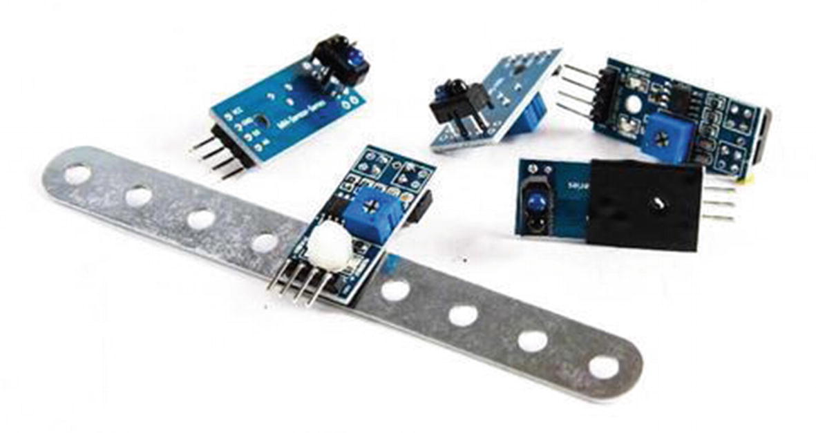
IR sensors for line following
Connecting an IR Sensor
The sensor that I used for my robot is a four-pin variant of the common three-pin IR sensor. The three-pin sensors are digital and apply a threshold to the analog signal of the sensor to return a high or a low signal. The four-pin version uses the same threshold setting to return a digital signal, but it also has an additional pin that provides the analog reading. Let’s walk through using both signals.
The sensors I use are a little different than most. They were specifically designed for use in line-following applications. As such, the return values are inverted. This means that rather than providing high numbers when the reflectance is high, it returns low numbers. In the same vein, the digital signal is also inverted. A high value indicates the presence of a line, and a low value indicates white space. When you run the next exercise, don’t be surprised if your results are different. We are looking for fairly consistent behavior.
We will connect the four-pin sensor to the Arduino and use the serial monitor to see the output of the sensor. We could use a digital pin for the high/low signal and an analog pin for the analog sensor, but to make the wiring easier, we use two of the analog pins. The analog pin connected to the digital output is used in digital mode, so it acts exactly like the other pins.
Since the Arduino is now mounted on the robot, let’s use the sensor shield for the connections. Also, I’m not going to disconnect the ultrasonic rangefinders. The sketch for the IR sensors doesn’t use those pins, so there is no reason to disconnect them.
- 1.
Using a female-to-female jumper, connect the ground pin of the sensor to the ground pin of the A0 three-pin header.
- 2.
Connect the VCC pin of the sensor to the voltage pin of the three-pin header A0. This is the middle pin.
- 3.
Connect the analog pin to the signal pin for A0. (On my sensor, the analog pin is labeled A0.)
- 4.
Connect the sensor’s digital pin to A1’s signal pin. (On my sensor, it is labeled D0.)
- 5.
Create a new sketch in the Arduino IDE.
- 6.
Save the sketch as IR_test.
- 7.Enter the following code:int analogPin = A0;int digitalPin = A1;float analogVal = 0.0;int digitalVal = 0;void setup() {pinMode(analogPin, INPUT);pinMode(digitalPin, INPUT);Serial.begin(9600);}void loop() {analogVal = analogRead(analogPin);digitalVal = digitalRead(digitalPin);Serial.print("analogVal: "); Serial.print(analogVal);Serial.print(" - digitalVal: "); Serial.println(digitalVal);delay(500);}
- 8.
Move the sensor over the white area of your surface. The sensor needs to be very close to the surface without touching it.
- 9.
Note the values being returned. (I got analog values in the 3045 range. My digital value was 0.)
- 10.
Move the sensor over the line or another black area on the surface.
- 11.
Note the values. (I got analog values in the 700900 range. The digital value was 1.)
You should have received very different values between the light and dark areas of your surface. You can see how this is easily translated into very useful functionality.
Mounting the IR Sensors
Next , we’re going to mount the sensors onto the robot to do something useful. Again, since your build may vary greatly from mine, I will walk through what I did to connect the sensors. If you’ve been faithfully following along, then you should replicate what I’ve done. If not, then this is where robotics starts to get creative. You need to determine how to mount the sensors onto your robot. Take a look at my solution to get an idea of what you’re looking for.
To mount the sensors, I turned (once again) to the parts in the Erector Set. These parts are incredibly convenient and easy to use. In this case, I used one of the bars and the same angle bracket used to mount the ultrasonic rangefinders. In fact, by using the angle bracket, I extended that assembly to bring the IR sensors closer to the ground.
In attempting to then mount the IR sensors, I encountered an issue. The hole for mounting the sensor is between two surface mount resistors. This means a metal standoff would likely cause a short. The nylon standoffs in my inventory are too large to lay flat in that space. I can use spacers and a long screw, but the spacers are too narrow and won’t sit straight against the holes in the mounting bar. Adding washers brings the sensors too close to the ground.
Mounting the IR sensors on a bar. Electrical tape protects the leads from shorting
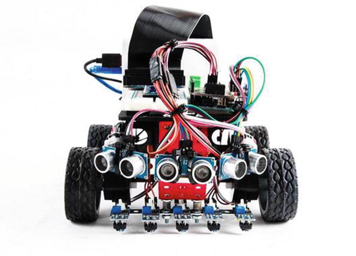
The completed robot with IR sensors mounted and wired
The Code
This project, like the last, uses the Arduino as the GPIO device. The majority of the logic is performed by the Raspberry Pi. We will read the IR sensors in 10-millisecond intervals, 100 times per second. These values are passed to the Raspberry Pi to work with. As you saw in an earlier exercise, reading the sensors is very easy, so the Arduino code is pretty light.
The Pi side is significantly more complex. First, we have to calibrate the sensors. Then, once calibrated, we have to write an algorithm that uses the readings from the sensors to keep the robot on a line. This may be more complicated than you expect. Later in this chapter, we look at a good solution, but for now, we’ll use a more direct approach.
Arduino Code
- 1.
Start a new sketch in the Arduino IDE.
- 2.
Save the sketch as line_follow1.
- 3.Enter the following code:int ir1Pin = A0;int ir2Pin = A1;int ir3Pin = A2;int ir4Pin = A3;int ir5Pin = A4;int ir1Val = 0;int ir2Val = 0;int ir3Val = 0;int ir4Val = 0;int ir5Val = 0;void setup() {pinMode(ir1Pin, INPUT);pinMode(ir2Pin, INPUT);pinMode(ir3Pin, INPUT);pinMode(ir4Pin, INPUT);pinMode(ir5Pin, INPUT);Serial.begin(9600);}void loop() {ir1Val = analogRead(ir1Pin);ir2Val = analogRead(ir2Pin);ir3Val = analogRead(ir3Pin);ir4Val = analogRead(ir4Pin);ir5Val = analogRead(ir5Pin);Serial.print(ir1Val); Serial.print(",");Serial.print(ir2Val); Serial.print(",");Serial.print(ir3Val); Serial.print(",");Serial.print(ir4Val); Serial.print(",");Serial.println(ir5Val);delay(100);}
- 4.
Save and upload the sketch.
This sketch is very straightforward. All we are doing is reading each of the five sensors and printing the results to the serial port.
Python Code
Most of the processing is done on the Pi. The first thing we need to do is calibrate the sensors to get the high and low values. To do that, we need to sweep the sensors back and forth over the line while we read the values from each sensor. We are looking for the highest and lowest values. Once we’ve done a few passes over the line, we should have good values to work with.
With the sensors calibrated, it’s time to start moving. Drive the robot forward. As long as the line is detected by the middle sensor, just keep driving forward. If one of the sensors to the left or right reads the line, make a slight correction the opposite direction to realign. If one of the outside sensors reads the line, make a more dramatic correction. This keeps the robot following along the line and handling easy turns.
To run this code properly, make a line for it to follow. There are several ways to do this. If you happen to have a white tile floor, then you can put electrical tape directly on it. Electrical tape lifts from the tile without damaging it. Otherwise, you can use sheets of paper, poster board, or foam core board like those used for science fair displays. Again, use electrical tape to mark the line. Be sure to add some curves.
- 1.
Open a new file in the Thonny IDE.
- 2.
Save the file as line_follower1.py.
- 3.
Import the necessary libraries:
- 4.
Create the motor objects as a list of motors:
# create motor objectkit = MotorKit()# create motor listmotors = [kit.motor1, kit.motor2, kit.motor3, kit.motor4] - 5.
Define the variables needed to control the motors. Again, let’s create lists:
# motor multipliersmotorMultiplier = [1.0, 1.0, 1.0, 1.0, 1.0]# motor speedsmotorSpeed = [0,0,0,0] - 6.
Open the serial port:
# open serial portser = serial.Serial('/dev/ttyAMA0', 9600) - 7.
Define the necessary variables. As with the motors, define some of the variables as lists. (This pays off later in the code. I promise.)
# create variables# sensorsirSensors = [0,0,0,0,0]irMins = [0,0,0,0,0]irMaxs = [0,0,0,0,0]irThesh = 50# speedsspeedDef = 1.0leftSpeed = speedDefrightSpeed = speedDefcorMinor = 0.25corMajor = 0.5turnTime = 0.5defTime = 0.01driveTime = defTimesweepTime = 1000 #duration of a sweep in milliseconds - 8.
Define the function to drive the motors. Though similar, this code is different from the roamer function:
def driveMotors(leftChnl = speedDef, rightChnl = speedDef,duration = defTime):# determine the speed of each motor by multiplying# the channel by the motors multipliermotorSpeed[0] = leftChnl * motorMultiplier[0]motorSpeed[1] = leftChnl * motorMultiplier[1]motorSpeed[2] = rightChnl * motorMultiplier[2]motorSpeed[3] = rightChnl * motorMultiplier[3] - 9.
Iterate the motor list to set the speed. Also, iterate the motorSpeed list:
# set each motor speed. Since the speed can be a# negative number, we take the absolute valuefor x in range(4):motors[x].setSpeed(abs(int(motorSpeed[x]))) - 10.
Run the motors:
# run the motors. if the channel is negative, run# reverse. else run forwardif(leftChnl < 0):motors[0].throttle(-motorSpeed[0])motors[1].throttle(-motorSpeed[1])else:motors[0].throttle(motorSpeed[0])motors[1].throttle(motorSpeed[1])if (rightChnl < 0):motors[2].throttle(motorSpeed[2])motors[3].throttle(motorSpeed[3])else:motors[2].throttle(-motorSpeed[2])motors[3].throttle(-motorSpeed[3])# wait for durationtime.sleep(duration) - 11.Define the function to read the IR sensor values from the serial stream and parse them:def getIR():# read the serial portval = ser.readline().decode('utf-8')# parse the serial stringparsed = val.split(',')parsed = [x.rstrip() for x in parsed]
- 12.Iterate the irSensors list to assign the parsed values, and then flush any remaining bytes from the serial stream:if(len(parsed)==5):for x in range(5):irSensors[x] = int(parsed[x]+str(0))/10# flush the serial buffer of any extra bytesser.flushInput()
- 13.Define the function to calibrate the sensors. The calibration goes through four complete cycles to read the minimum and maximum values from the sensor:def calibrate():# set up cycle count loopdirection = 1cycle = 0# get initial values for each sensor# and set initial min/max valuesgetIR()for x in range(5):irMins[x] = irSensors[x]irMaxs[x] = irSensors[x]
- 14.Loop through the cycle five times to assure that you get four full-cycle readings:while cycle < 5:#set up sweep loopmillisOld = int(round(time.time()*1000))millisNew = millisOld
- 15.
For the duration of sweepTime, drive the motors and read the IR sensors:
while((millisNew-millisOld)<sweepTime):leftSpeed = speedDef * directionrightSpeed = speedDef * -direction# drive the motorsdriveMotors(leftSpeed, rightSpeed, driveTime)# read sensorsgetIR() - 16.
Update irMins and irMaxs if the sensor values are below or above the current irMins or irMaxs values:
# set min and max values for each sensorfor x in range(5):if(irSensors[x] < irMins[x]):irMins[x] = irSensors[x]elif(irSensors[x] > irMaxs[x]):irMaxs[x] = irSensors[x]millisNew = int(round(time.time()*1000)) - 17.
After one cycle, change motor directions and increment the cycle value:
# reverse directiondirection = -direction# increment cyclescycle += 1 - 18.
When the cycles have completed, drive the robot forward:
# drive forwarddriveMotors(speedDef, speedDef, driveTime) - 19.Define the followLine function:def followLine():leftSpeed = speedDefrightSpeed = speedDefgetIR()
- 20.
Define the behavior based on the sensor readings. If the line is detected by the far-right or far-left sensor, do a major correction in the other direction. If the inner-right or inner-left sensor detects the line, do a minor correction in the other direction; else, drive straight:
# find line and correct if necessaryif(irMaxs[0]-irThresh <= irSensors[0]<= irMaxs[0]+irThresh):leftSpeed = speedDef-corMajorelif(irMaxs[1]-irThresh <= irSensors[1]<= irMaxs[1]+irThresh):leftSpeed = speedDef-corMinorelif(irMaxs[3]-irThresh <= irSensors[3]<= irMaxs[3]+irThresh):rightSpeed = speedDef-corMinorelif(irMaxs[4]-irThresh <= irSensors[4]<= irMaxs[4]+irThresh):rightSpeed = speedDef-corMajorelse:leftSpeed = speedDefrightSpeed = speedDef# drive the motorsdriveMotors(leftSpeed, rightSpeed, driveTime) - 21.
Enter the code to run the program:
# execute programtry:calibrate()while 1:followLine()time.sleep(0.01)except KeyboardInterrupt:kit.motor1.throttle(0)kit.motor2.throttle(0)kit.motor3.throttle(0)kit.motor4.throttle(0) - 22.
Save the code.
- 23.
Place the robot on the line. The robot should be aligned so that the line runs between the left and right wheels and the center sensor is directly over it.
- 24.
Run the program.
Your robot should now follow along the line, making corrections if it starts to wander off the line. You probably need to play with the corMinor and corMajor variables to fine-tune the behavior.
What we executed here is known as proportional control. This is the simplest form of control algorithm. The basic logic behind it is that if your robot is a little off course, apply a little correction. If the robot is a lot off course, apply a lot more correction. The amount of correction applied to the robot is determined by how big the error is.
With proportional control alone, the robot tries really hard to follow the line. It may even succeed; however, you will note how it zigzags along the line. This behavior may be reduced over time and become smooth; however, when you introduce a curve, the erratic behavior starts all over again. More likely, your robot overcorrected and wandered off in a random direction, leaving the line far behind.
There is a better way to control the robot. In fact, there are several better ways, all from a field of study called control loops. Control loops are algorithms to improve the response of a machine or program. Most of them use the difference between the current state and a desired state to control the machine. This difference is called the error.
Let’s look at once such control system next.
Understanding PID Control
To better control the robot, you are going to learn about PID control, and I’ll try to discuss it without getting math heavy. The PID controller is one of the most widely used control loops because of its versatility and simplicity. We’ve actually already used part of a PID controller: proportional control. The remaining parts help smooth the reaction and provide a better response.
Control Loops
The PID controller is a member of a group of algorithms called control loops . The purpose of a control loop is to use input from a measured process to make changes to a control, or controls, to compensate for differences between the current state and a desired state. There are many different types of control loops. In fact, control loops are a whole area of study called control theory . For our purposes, we really only care about one: proportional, integral, and derivative—or PID.
Proportional, Integral, and Derivative Control
According to Wikipedia, a “PID controller continuously calculates an error value (e(t)) as the difference between a desired setpoint and a measured process variable and applies a correction based on proportional, integral, and derivative terms. PID is an initialism for Proportional-Integral-Derivative, referring to the three terms operating on the error signal to produce a control signal.”
The purpose of the controller is to apply incremental adjustments to some output to achieve the desired result. In our application, we use the feedback from IR sensors to apply changes to our motors. The desired behavior is a robot that keeps centered on a line as it moves forward. This process can be used with any sensors and outputs, however; for instance, PID is used in multirotor platforms to remain level and maintain stability.
As the name implies, the PID algorithm actually consists of three parts: proportional, integral, and derivative. Each part is a type of control; however, if used independently, the resulting behavior would be erratic and difficult to predict.
Proportional Control
In proportional control , the amount of change is set based entirely on the size of the error. The larger the error, the more change is applied. A purely proportional control would reach a zero-error state, but has difficulty dealing with drastic changes, which results in heavy oscillation.
Integral Control
Integral control considers not only the error but also the time that it has persisted. The amount of change applied to compensate for the error increases over time. A purely integral control could bring the device to a zero-error state, but it reacts slowly and tends to overcompensate and oscillate.
Derivative Control
Derivative control does not consider the error, and therefore it can never bring the device to a zero-error state. It does try to reduce the change in error to zero, however. If too much compensation is applied, the algorithm overshoots and then applies another correction. The process continues in this manner, producing a pattern of constantly increasing or decreasing corrections. Although a state of decreasing oscillation is considered “stable,” the algorithm never reaches a truly zero-error state.
Bringing Them Together
The PID controller is simply the sum of the three methods. By bringing them together, the algorithm aims to produce a smooth correcting process that brings the error to zero. Time for a little bit of math.
Let’s start by defining some variables.
e(t) is the error in time, where (t) is time, or the present.
Kp is a parameter representing the proportional gain. When we start coding, this is the proportional variable.
Ki is the integral gain parameter. It is also a variable.
Kd is the derivative gain parameter. And you guessed it, yet another variable.
τ represents integrated values over time. I’ll get to that.


That’s it for the math. Fortunately, we don’t have to solve it ourselves. Python makes it very easy. However, it is important to understand what is happening inside the equation. There are three parameters to adjust to fine-tune the PID controller. By understanding how these parameters are used, you will be able to determine which ones need adjusting and when.
Implementing the PID Controller
To implement the controller, we need to know a few things. What is our desired outcome? What are our inputs? What are our outputs?
The goal is to improve the performance of our line-following robot. So our desired outcome is that the line remains in the center of the robot while it drives forward.
Our inputs are the IR sensors. When an outer sensor is over a dark area (the line), the error is twice that of the inner sensors. In this way, we’ll know whether the robot is a little off-center or a lot off-center. Also, the two left sensors will have a negative value, and the right sensors will have a positive value, so we will know which direction is off.
Finally, our outputs are the motors. More accurately, our output is the difference in speed between the left and right motor channels.
The Code
The code for this exercise is a modification of the earlier code. In fact, the Arduino code does not need to change at all. It’s the logic we are implementing on the Raspberry Pi that is updated.
Raspberry Pi Code
- 1.
Open the file line_follower1 in the Thonny IDE.
- 2.
Create a new file and save the file as line_follower2.py.
- 3.
Copy the code from line_follower1 and paste it to line_follower2.
- 4.In the variables section, under #sensors, add the following code:# PIDsensorErr = 0lastTime = int(round(time.time()*1000))lastError = 0target = 0kp = 0.5ki = 0.5kd = 1
- 5.Create the PID function:def PID(err):# check if variables are defined before use# the first time the PID is called these variables will# not have been definedtry: lastTimeexcept NameError: lastTime = int(round(time.time()*1000)-1)try: sumErrorexcept NameError: sumError = 0try: lastErrorexcept NameError: lastError = 0# get the current timenow = int(round(time.time()*1000))duration = now-lastTime# calculate the errorerror = target - errsumError += (error * duration)dError = (error - lastError)/duration# calculate PIDoutput = kp * error + ki * sumError + kd * dError# update variableslastError = errorlastTime = now# return the output valuereturn output
- 6.Replace the followLine function with this:def followLine():leftSpeed = speedDefrightSpeed = speedDefgetIR()prString = ''for x in range(5):prString += ('IR' + str(x) + ': ' + str(irSensors[x]) + ' ')print prString# find line and correct if necessaryif(irMaxs[0]-irThresh <= irSensors[0]<= irMaxs[0]+irThresh):sensorErr = 2elif(irMaxs[1]-irThresh <= irSensors[1]<= irMaxs[1]+irThresh):sensorErr = 1elif(irMaxs[3]-irThresh <= irSensors[3]<= irMaxs[3]+irThresh):sensorErr = -1elif(irMaxs[4]-irThresh <= irSensors[4]<= irMaxs[4]+irThresh):sensorErr = -1else:sensorErr = 0# get PID resultsratio = PID(sensorErr)# apply ratioleftSpeed = speedDef * ratiorightSpeed = speedDef * -ratio# drive the motorsdriveMotors(leftSpeed, rightSpeed, driveTime)
- 7.
Save the file.
- 8.
Place the robot on the line.
- 9.
Run the code.
Once again, your robot should be trying to follow the line. If it is having problems doing so, start working with the Kp, Ki, and Kd variables. These variables need to be fine-tuned for the best results. Every robot is different.
Summary
In this chapter, we added some new sensors to the robot. The IR sensors were applied in a line-following application. They can also be used to detect the edge of a surface. This functionality is useful if you want to prevent your robot from driving off a table or downstairs.
Our first implementation of line following used a basic proportional control to steer the robot. This was functional, but barely. A much better way of doing this was the use of a control loop called the PID controller, which uses several factors, including error over time, to make the corrections smoother. You learned that you can adjust the ID settings by using the PID parameters represented in our code, with the Kp, Ki, and Kd variables. With the proper values, the oscillation can be eliminated completely, causing the robot to follow the line smoothly.