We’ve come a long way since the first chapters introducing the Raspberry Pi. At this point, you have learned about the Pi and the Arduino. You’ve learned how to program both boards. You’ve worked with sensors and motors. You’ve built your robot and programmed it to roam around and to follow a line.
However, to be completely honest, you haven’t really needed the power of the Raspberry Pi. In fact, it’s been a bit of hindrance. Everything you’ve done with the robot—roaming and line following—you could do just well with the Arduino and without the Pi. It’s now time to show the real power of the Pi and to learn why you want to use it in your robot.
In this chapter, we’re going to do something you can’t do with the Arduino alone. We are going to connect a simple web camera and start working with what is commonly known as computer vision.
Computer Vision
Computer vision is a collection of algorithms that allow a computer to analyze an image and extract useful information. It is used in many applications, and it is rapidly becoming a part of everyday life. If you have a smartphone, chances are you have at least one app that uses computer vision. Most new moderate to high-end cameras have facial detection built in. Facebook uses computer vision for facial detection. Computer vision is used by shipping companies to track packages in their warehouses. And, of course, it’s used in robotics for navigation, object detection, object avoidance, and many other behaviors.
It all starts with an image. The computer analyzes an image to identify lines, corners, and a broad area of color. This process is called feature extraction , and it is the first step in virtually all computer vision algorithms. Once the features are extracted, the computer can use this information for many different tasks.
Facial recognition is accomplished by comparing the features against XML files containing feature data for faces. These XML files are called cascades . They are available for many different types of objects, not just faces. This same technique can be used for object recognition. You simply provide the application with feature information for the objects that interest you.
Computer vision also incorporates video. Motion tracking is a common application for computer vision. To detect motion, the computer compares individual frames from a stationary camera. If there is no motion, the features will not change between frames. So, if the computer identifies differences between frames, there is most likely motion. Computer vision–based motion tracking is more reliable than IR sensors, such as the PIR sensor discussed in Chapter 8.
An exciting, recent application of computer vision is augmented reality. The extracted features from a video stream can be used to identify a unique pattern on a surface. Because the computer knows the pattern, it can easily calculate the angle of the surface. A 3D model is then superimposed over the pattern. This 3D model could be something physical, like a building, or it could be a planar object with two-dimensional text. Architects use this technique to show clients what a building would look like against a skyline. Museums use it to provide more information about an exhibit or an artist.
All of these are examples of computer vision in modern settings. But the list of applications is too large to discuss in depth here, and it keeps growing.
OpenCV
Just a few years ago, computer vision was not really accessible to the hobbyist. It required a lot of heavy math and even heavier processing. Computer vision projects were generally done using laptops, which limited its application.
OpenCV has been around for a while. In 1999, Intel Research established an open standard for promoting the development of computer vision. In 2012, it was taken over by the nonprofit OpenCV Foundation. You can download the latest version at their website. It takes a little extra effort to get it running on the Raspberry Pi, however. We’ll get to that shortly.
OpenCV is written natively in C++; however, it can be used in C, Java, and Python. We are interested in the Python implementation.
Installing OpenCV
As with the Raspberry Pi OS, there are two methods to install OpenCV: the easy way, using Python’s pip install method, and the hard way, compiling the packages from source code. Unlike Raspberry Pi OS, the hard way for OpenCV is significantly more complicated and, frankly, difficult. I will present both, but strongly suggest using the easy way.
Installing the Prerequisites
- 1.
Log on to your Raspberry Pi.
- 2.
Open a terminal window on the Pi.
- 3.
Make sure that the Raspberry Pi is updated:
sudo apt-get updatesudo apt-get upgrade - 4.
These commands install the prerequisites for building OpenCV. Because we are doing this on a fresh installation of Raspberry Pi OS, it is likely some of these may already be installed and using the most recent version:
sudo apt-get install build-essential git cmake pkg-configsudo apt-get install libjpeg-dev libtiff5-dev libjasper-dev libpng12-devsudo apt-get install libavcodec-dev libavformat-dev libswscale-dev libv4l-devsudo apt-get install libxvidcore-dev libx264-devsudo apt-get install libfontconfig1-dev libcairo2-devsudo apt-get install libgdk-pixbuf2.0-dev libpango1.0-devsudo apt-get install libgtk2.0-devsudo apt-get install libatlas-base-dev gfortransudo apt-get install libhdf5-dev libhdf5-serial-dev libhdf5-103sudo apt-get install libqtgui4 libqtwebkit4 libqt4-test python3-pyqt5
Installing OpenCV with pip install
Python has a built-in system for installing packages for use in Python called the preferred installer program, or pip. In order to use it, however, you will need to use the command line. This is, by far, the easiest and fastest method to complete the installation. However, the version tends to lag behind the most current version. It also does not contain the full library.
- 1.
Log on to your Raspberry Pi.
- 2.
Open a terminal window on the Pi.
- 3.Install OpenCV:sudo pip install opencv-contrib-python
- 4.
Celebrate the successful installation of OpenCV on your Pi.
Compiling OpenCV from Source Code
We will install OpenCV on the Raspberry Pi by compiling the package from scratch. This method will give you the most complete installation. You want to make sure that your Raspberry Pi is plugged into a charger rather than the battery pack and give yourself plenty of time for the installation.
- 1.
Log on to your Raspberry Pi.
- 2.
Open a terminal window on the Pi.
- 3.
Download the OpenCV source code and the OpenCV contributed files. The contributed files contain a lot of functionality not yet rolled into the main OpenCV distribution:
cd ~wget -O opencv.zip https://github.com/opencv/opencv/archive/4.4.0.zipwget -O opencv_contrib.zip https://github.com/opencv/opencv_contrib/archive/4.4.0.zipunzip opencv.zipunzip opencv_contrib.zipmv opencv-4.4.0 opencvmv opencv_contrib-4.4.0 opencv_contrib - 4.
Install the Python development libraries and pip:
sudo apt-get install python3-devwget https://bootstrap.pypa.io/get-pip.pysudo python get-pip.py - 5.
Make sure that NumPy is installed:
pip install numpy - 6.
Increase the memory allocated for swap. The compilation of these libraries is very memory intensive. The likelihood of your Pi hanging due to memory issues is greatly reduced by doing this. Open the file /etc/dphys-swapfile:
sudo nano /etc/dphys-swapfile
- 7.
Use the arrow keys to navigate the text and update the line:
CONF_SWAPSIZE=100toCONF_SWAPSIZE=2048 - 8.
Save and exit the file by pressing Ctrl-X, followed by Y and then Enter.
- 9.
Restart the swap service:
sudo /etc/init.d/dphys-swapfile stopsudo /etc/init.d/dphys-swapfile start - 10.Prepare the source code for compiling:cd ~/opencvmkdir buildcd buildcmake -D CMAKE_BUILD_TYPE=RELEASE-D CMAKE_INSTALL_PREFIX=/usr/local-D OPENCV_EXTRA_MODULES_PATH=~/opencv_contrib/modules-D ENABLE_NEON=ON-D ENABLE_VFPV3=ON-D BUILD_TESTS=OFF-D INSTALL_PYTHON_EXAMPLES=OFF-D OPENCV_ENABLE_NONFREE=ON-D CMAKE_SHARED_LINKER_FLAGS=-latomic-D BUILD_EXAMPLES=OFF ..
- 11.
Now let’s compile the source code. This part is going to take a while:
make -j4 - 12.
If you attempted the –j4 switch and it failed, somewhere around hour 4, enter the following lines:
make cleanmake - 13.
With the source code compiled, you can now install it:
sudo make installsudo ldconfig - 14.
Set your swap memory back to its default value:
sudo nano /etc/dphys-swapfile
- 15.
Use the arrow keys to navigate the text and update the line:
CONF_SWAPSIZE=2048toCONF_SWAPSIZE=100 - 16.
Save and exit the file by pressing Ctrl-X, followed by Y and then Enter.
- 17.
Test the installation by opening a Python command line:
python - 18.
Import OpenCV:
>>>import cv2
You should now have an operating version of OpenCV installed on your Raspberry Pi. If the import command did not work, you need to determine why it did not install. The Internet is your guide for troubleshooting.
Selecting a Camera
Before we can really put OpenCV to work on our robot, we need to install a camera. There are a couple of options with the Raspberry Pi: the Pi Camera or a USB web camera.
The Pi Camera connects directly to a port designed specifically for it. Once connected, you need to go into raspi-config and enable it. The advantage of the Pi Camera is that it is a little bit faster than a USB camera because it is connected directly to the board. It does not go through the USB. This gives it a slight advantage.
Most of the Pi Cameras come with a short, 6-inch ribbon cable. Due to the placement of the Raspberry Pi on our robot, this is insufficient. It is possible to order longer cables. Adafruit has a couple of options. But, for this project, we will use a simple web camera.
USB cameras are readily available at any electronics retailer. There are many options online, as well. For this basic application, we won’t need anything particularly robust. Any camera that can provide a decent image will do. Having a high resolution is not a concern, either. Since we are running the camera with the limited resources of the Raspberry Pi, a lower resolution would actually help performance. Remember, OpenCV analyzes each frame pixel by pixel. The more pixels there are in an image, the more processing it has to do.

Creative Live! Cam Sync HD
Installing the Camera
Most web cams are mounted on top of a monitor. They usually have a folding clamp to provide support for the camera when on the monitor. Unfortunately, these clamps are usually molded as part of the camera’s body and can’t be removed without damaging it. This certainly holds true with the Live! Cam Sync. So, once again, a little creativity comes into play.

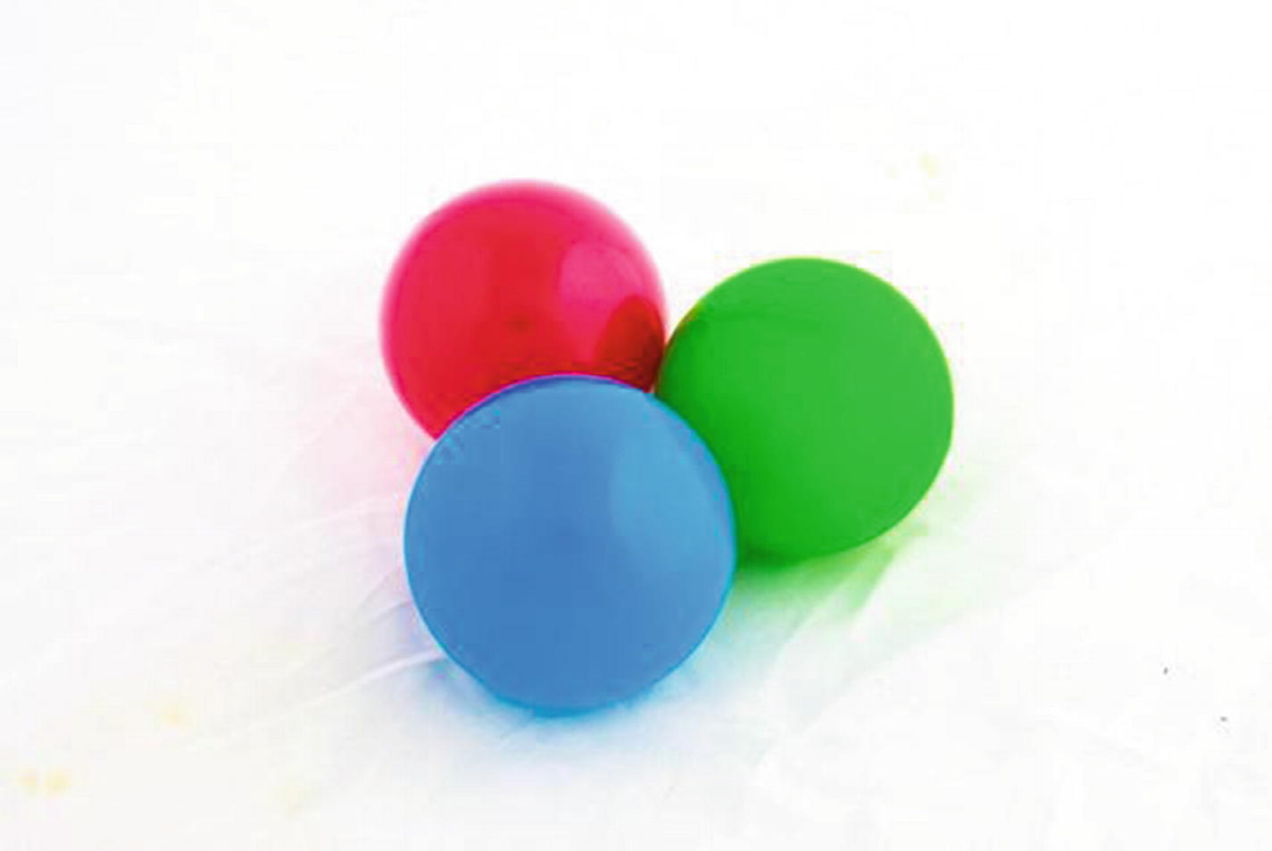
Camera mounted on the robot
OpenCV Basics
OpenCV has many capabilities. It boasts more than 500 libraries and thousands of functions. It is a very big subject—too large a subject to cover in one chapter. I’ll discuss the basics needed to perform some simple tasks on your robot.
I said simple tasks. These tasks are only simple because OpenCV abstracts the monumental amount of math that is happening in the background. When I consider the state of hobby robotics a few short years ago, I find it amazing to be able to easily access even the basics.
The goal is to build a robot that can identify a ball and move toward it by the end of this chapter. The functions I cover will help us achieve that goal. I strongly suggest spending time going through some of the tutorials at the OpenCV website (https://opencv.org).
In the code discussions in this chapter, I assume this has been done. A function prefixed with cv2 is an OpenCV function. If it’s prefixed with np, it is a NumPy function. It’s important to make this distinction in the event that you want to expand on what you read in this book. OpenCV and NumPy are two separate libraries, but OpenCV frequently uses NumPy.
Working with Images
In this section, you learn how to open images from a file and how to capture live video from the camera. We’ll then take a look at how to manipulate and analyze the images to get usable information out of them. Specifically, we’ll work on how to identify a ball of a particular color and track its position in the frame.
But first, we have a bit of a chicken-or-egg issue. We need to see the results of our image manipulation in all the exercises. To do that, we need to start with how to display an image. It is something that we’ll use extensively, and it’s very easy to use. But I want to make sure that I cover it first, before you learn how to capture an image.
Displaying an Image
It’s actually very easy to display an image in OpenCV. The imshow() function provides this functionality. This function is used with both still and video images, and the implementation does not change between them. The imshow() function opens a new window to display the image. When you call it, you have to provide a name for the window as well as the image or frame that you want to display.
This is an important point about how OpenCV works with video. Because OpenCV treats a video as a series of individual frames, virtually all the functions used to modify or analyze an image apply to a video. This obviously includes imshow().
As you can see, the code is the same. Again, this is because OpenCV treats video as a series of individual frames. In fact, video capture depends on a loop to continuously capture the next frame. So in essence, displaying a still image from a file and an individual frame from the camera is exactly the same thing.
We use imshow() and waitKey() extensively throughout this chapter.
Capturing Images
There are several sources for the images needed to work with OpenCV, all of which are a variation of two factors: file or camera and still or video. For the most part, we are only concerned with video from a camera since we are using OpenCV for navigation purposes. But there are advantages to all the methods.
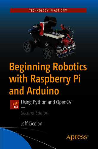
Opening a still image file is an excellent way to learn new techniques, especially when you are working with specific aspects of computer vision. For example, if you are learning how to use filters to identify a ball of a certain color, using a still image that consists of three different colored balls (and nothing else) allows you to focus on that specific goal without having to worry about the underlying framework for capturing a live video stream. Oh, and that was a bit of foreshadowing, if you hadn’t picked up on that.
The techniques learned from capturing a still image with a camera can be applied to a live environment. It allows you to hone or fine-tune the code by using an image that contains elements of the real world.
Obviously, capturing live video is what we’re after for use in the robot. The live video stream is what we’ll use to identify our target object and then navigate to it. As your computer vision experience grows, you will probably add motion detection or other methods to your repertoire. Since the purpose of the camera on the robot is to gather environmental information in real time, live video is required.
Video from a file is also very useful for the learning process. You may want to capture live video from your robot and save it to a file for later analysis. Let’s say that you are working on your robot project in whatever spare time you are able to find throughout the day. You can port your laptop with you, but carting a robot around is a different story. So, if you record the video from your robot, you can work on your computer vision algorithms without having the robot with you.
Remember, one of the great things about Python and OpenCV is that they’re abstracted and platform independent, for the most part. So the code you write on your Windows machine ports to your Raspberry Pi.
Going on a business trip and expecting some downtime in the hotel? Heading to the family’s place for the holidays and needing to get away every once in a while? Slipping in a little robot programming during your lunch hour or between classes? Use the recorded video with a local instance of Python and OpenCV, and work on your detection algorithm. When you get home, you can transfer that code to your robot and test it live.
In this section, we use the first three techniques. I show you how to save and open video files, but for the most part, we’ll use stills to learn the detection algorithm and the live video to learn tracking.
Opening an Image File
OpenCV makes working with images and files remarkably easy, especially considering what is happening in the background to make these operations possible. Opening an image file is no different. We use the imread() function to open image files from local storage. The imread() function takes two parameters: file name and color type flag. The file name is obviously required to open the file. The color type flag determines whether to open the image in color or grayscale.
- 1.
Open the Thonny IDE and create a new file.
- 2.
Save the file as open_image.py.
- 3.
Enter the following code:
import cv2img = cv2.imread('color_balls_small.jpg')cv2.imshow('image',img)cv2.waitKey(0) - 4.
Save the file.
- 5.
Open a terminal window.
- 6.
Navigate to the folder in which you saved the file.
- 7.
Enter python open_image.py and press Return.
Three colored balls
Due to the way Thonny interacts with the GUI system on Linux-based machines, the image window will not close properly if you were to run the code directly from Thonny. However, by running the code from the terminal, we do not have this issue.
Capturing Video
Capturing video with your camera is a little different from opening a file. There are a few more steps to use video. One change is that we have to use a loop to get multiple frames; otherwise, the OpenCV will only capture a single frame, which is not what we want. An open while loop is generally used. This captures the video until we actively stop it.
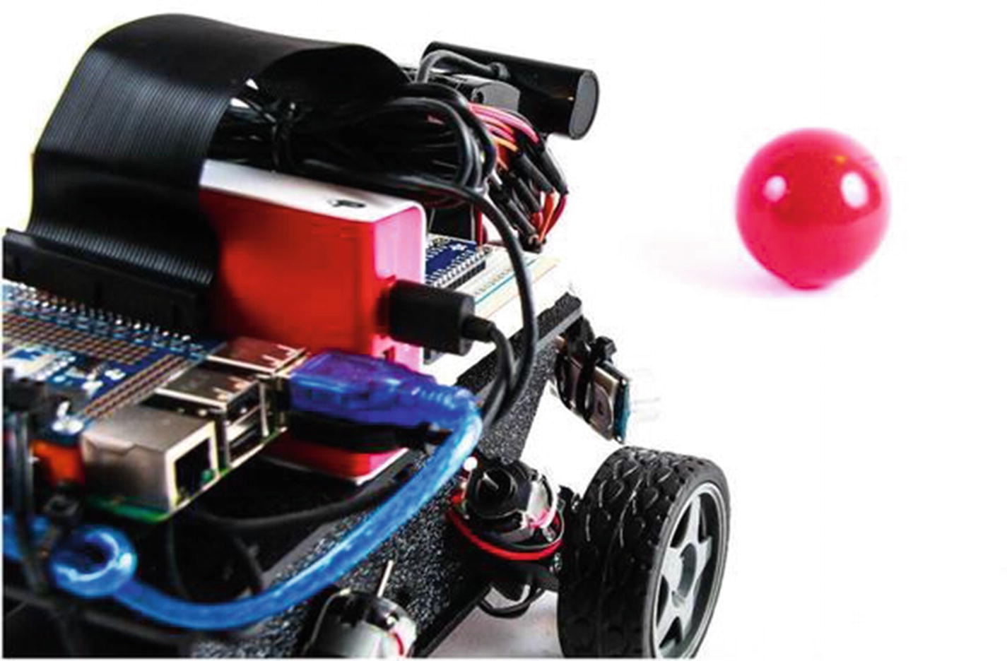
Ball positioned in front of the robot for testing
To capture the video from the camera, we will create a videoCapture() object and then use the read() method in a loop to capture the frames. The read() method returns two objects: a return value and an image frame. The return value is simply an integer verifying the success or failure of the read. If the read is successful, the value is 1; otherwise, the read failed and it returns 0. To prevent errors that cause your code to error, you can test to see if the read is successful.
We care about the image frame. If the read is successful, an image is returned. If it was not, then a null object is returned in its place. Since a null object cannot access OpenCV methods, the instant you try to modify or manipulate the image, your code will crash. This is why it’s a good idea to test for the success of the read operation.
Viewing the Camera
- 1.
Open the Thonny IDE and create a new file.
- 2.
Save the file as view_camera.py.
- 3.
Enter the following code:
import cv2import numpy as npcap = cv2.VideoCapture(0)while(True):ret,frame = cap.read()cv2.imshow('video', frame)if cv2.waitKey(1) & 0xff == ord('q'):breakcap.release()cv2.destroyAllWindows() - 4.
Save the file.
- 5.
Open a terminal window.
- 6.
Navigate to your working folder where the script is saved.
- 7.
Type sudo python view_camera.py.
This opens a window displaying what your camera sees. If you are using a remote desktop session to work on the Pi, you may see this warning message: Xlib: extension RANR missing on display :10. This message means that the system is looking for functionality not included in VNC server. It can be ignored.
If you are concerned about the refresh rate of the video image, keep in mind that we are asking an awful lot of the Raspberry Pi when we run several windows through a remote desktop session. If you connect a monitor and keyboard to access the Pi, it runs much faster. The video capture works faster if you run it with no visualization.
Recording Video
Recording a video is an extension of viewing the camera. To record, you have to declare the video codec that you will use and then set up the VideoWriter object that writes the incoming video to the SD card.
OpenCV uses the FOURCC code to designate the codec. FOURCC is a four-character code for a video codec. You can find more information about FOURCC at www.fourcc.org.
When creating the VideoWriter object, we need to provide some information. First, we have to provide the name of the file to save the video. Next, we provide the codec, followed by the frame rate and the resolution. Once the VideoWriter object is created, we simply have to write each frame to the file using the write() method of the VideoWriter object.
- 1.
Open the view_camera.py file in the Thonny IDE.
- 2.
Select File ➤ Save as and save the file as record_camera.py.
- 3.Update the code. In the following, the new lines are in bold:import cv2import numpy as npcap = cv2.VideoCapture(0)fourcc = cv2.VideoWriter_fourcc(*'XVID')vidWrite = cv2.VideoWriter('test_video.avi',fourcc, 20, (640,480))while(True):ret,frame = cap.read()vidWrite.write(frame)cv2.imshow('video', frame)if cv2.waitKey(1) & 0xff == ord('q'):breakcap.release()vidWrite.release()cv2.destroyAllWindows()
- 4.
Save the file.
- 5.
Open a terminal window.
- 6.
Navigate to your working folder where the script is saved.
- 7.
Type sudo python record_camera.py.
- 8.
Let the video run for a few seconds, and then press Q to end the program and close the window.
You should now have a video file in your working directory. Next, we’ll look at reading a video from a file.
There are a couple items to note in the code. When we created the VideoWriter object, we supplied the video resolution as a tuple. This is a very common practice throughout OpenCV. Also, we had to release the VideoWriter object. This closed the file from writing.
Reading Video from a File
Playing a video back from a file is exactly the same as viewing a video from a camera. The only difference is that rather than providing the index to a video device, we provide the name of the file to play. We will use the ret variable to test for the end of the video file; otherwise, we would get an error when there is no more video to play.
- 1.
Open the Thonny IDE and create a new file.
- 2.
Save the file as view_video.py.
- 3.
Enter the following code:
import cv2import numpy as npcap = cv2.VideoCapture('test_video.avi')while(True):ret,frame = cap.read()if ret:cv2.imshow('video', frame)if cv2.waitKey(1) & 0xff == ord('q'):breakcap.release()cv2.destroyAllWindows() - 4.
Save the file.
- 5.
Open a terminal window.
- 6.
Navigate to your working folder where the script is saved.
- 7.
Type sudo python view_video.py.
A new window opens. It displays the video file that we recorded in the previous exercise. When the end of the file is reached, the video stops. Press Q to end the program and close the window.
Image Transformations
Now that you know more about how to get an image, let’s take a look at some of the things that we can do with it. We will look at a few very basic operations. These operations were selected because they will help us reach our goal of tracking a ball. OpenCV is very powerful, and it has a lot more capabilities than I present here.
Flipping
Many times, the placement of the camera in a project is not ideal. Frequently, I’ve had to mount the camera upside down, or I’ve needed to flip the image for one reason or another.
Fortunately, OpenCV makes this very simple with the flip() method. The flip() method takes three parameters: the image to be flipped, the code indicating how to flip it, and the destination of the flipped image. The last parameter is only used if you want to assign the flipped image to another variable, but you can flip the image in place.
An image can be flipped horizontally, vertically, or both by providing the flipCode. The flipCode is positive, negative, or zero. Zero flips the image horizontally, a positive value flips it vertically, and a negative number flips it on both axes. More often than not, you will flip the image on both axes to effectively rotate it 180 degrees.
- 1.
Open the Thonny IDE and create a new file.
- 2.
Save the file as flip_image.py.
- 3.
Enter the following code:
import cv2img = cv2.imread('color_balls_small.jpg')h_img = cv2.flip(img, 0)v_img = cv2.flip(img, 1)b_img = cv2.flip(img, -1)cv2.imshow('image', img)cv2.imshow('horizontal', h_img)cv2.imshow('vertical', v_img)cv2.imshow('both', b_img)cv2.waitKey(0) - 4.
Save the file.
- 5.
Open a terminal window.
- 6.
Navigate to the folder in which you saved the file.
- 7.
Enter python flip_image.py and press Return.
Four windows open, each with a different version of the image file. Press any key to exit.
Resizing
You can resize an image. This is useful for reducing the resources needed to process an image. The larger the image, the more memory and CPU resources needed. To resize an image, we use the resize() method . The parameters are the image you are scaling, the desired dimensions as a tuple, and the interpolation.
Interpolation is the mathematical method used for determining how to handle the removal or addition of pixels. Remember, when working with images, you are really working with a multidimensional array that contains information for each point, or pixel, that makes up the image. When you reduce an image, you are removing pixels. When you enlarge an image, you are adding pixels. Interpolation is the method by which this occurs.
There are three interpolation options. INTER_AREA is best used for reduction. INTER_CUBIC and INTER_LINEAR are both good for enlarging an image, with INTER_LINEAR being the faster of the two. If an interpolation is not provided, OpenCV uses INTER_LINEAR as the default for both reducing and enlarging.
- 1.
Open the Thonny IDE and create a new file.
- 2.
Save the file as resize_image.py.
- 3.Enter the following code:import cv2img = cv2.imread('color_balls_small.jpg')x,y = img.shape[:2]resImg = cv2.resize(img, (y/2, x/2), interpolation = cv2.INTER_AREA)cv2.imshow('image', img)cv2.imshow('resized', resImg)cv2.waitKey(0)
- 4.
Save the file.
- 5.
Open a terminal window.
- 6.
Navigate to the folder in which you saved the file.
- 7.
Enter python resize_image.py and press Return.
Two windows should have opened. The first has the original image. The second displays the reduced image. Press any key to close the windows.
Working with Color
Color is obviously a very important part of working with images. As such, it is a very prominent part of OpenCV. There is a lot that can be done with color. We are going to focus on a few of the key elements needed to accomplish our end goal of identifying and chasing a ball with the robot.
Color Spaces
One of the key elements of working with color is color space, which describes how OpenCV expresses color. Within OpenCV, color is represented by a series of numbers. The color space determines the meaning of those numbers.
The default color space for OpenCV is BGR. This means every color is described by three integers between 0 and 255, which correspond to the three color channels—blue, green, and red, in that order. A color expressed as (255,0,0) has a maximum value in the blue channel, and both green and red are zero. This represents pure blue. Given this, (0,255,0) is green and (0,0,255) is red. The values (0,0,0) represent black, the absence of any color, and (255,255,255) is white.
If you’ve worked with graphics in the past, BGR is the opposite of what you’re likely used to. Most digital graphics are described in terms of RGB—red, green, and blue. So this may take a little getting used to.
There are many color spaces. The ones that we care about are BGR, RGB, HSV, and grayscale. We’ve already discussed the default color space, BGR, and the common RGB color space. HSV is hue, saturation, and value. Hue represents the color on a scale of 0–180. Saturation represents how far white the color is from 0 to 255. Value is a measure of how far from black the color is from 0 to 255. If both saturation and value are 0, the color is gray. A saturation and value of 255 is the brightest version of the hue.
Hue is a little trickier. It is on a scale of 0–180, where 0 and 180 are both red. This is where remembering the color wheel is important. If 0 and 180 meet at the top of the wheel in the middle of the red space, as you move clockwise around the wheel, hue = 30 is yellow, hue = 60 is green, hue = 90 is teal, hue = 120 is blue, hue = 150 is purple, and hue = 180 brings us back to red.
The one that you most frequently encounter is grayscale. Grayscale is exactly what it sounds like: the black-and-white version of an image. It is used by feature detection algorithms to create masks. We use it when we filter for objects.
To convert an image to a different color space, you use the cvtColor method. It takes two parameters: the image and the color space constant. The color space constants are built into OpenCV. They are COLOR_BGR2RGB, COLOR_BGR2HSV, and COLOR_BGR2GRAY. Do you see the pattern there? If you wanted to convert from the RGB color space to the HSV color space, the constant would be COLOR_RGB2HSV.
- 1.
Open the Thonny IDE and create a new file.
- 2.
Save the file as gray_image.py.
- 3.
Enter the following code:
- 4.
Save the file.
- 5.
Open a terminal window.
- 6.
Navigate to the folder in which you saved the file.
- 7.
Enter python gray_image.py and press Return.
This opens two windows: one with the original color image and one with the grayscale version. Click any key to exit the program and close the windows .
Color Filters
Filtering for a color takes remarkably little code, but at the same time, it can be a little frustrating because you’re generally not looking for a specific color but a color range. Colors are very rarely pure and of one value. This is why we want to be able to shift between color spaces. Sure, we could look for a red color in BGR. But to do that, we would need the specific range for each of the three values. And where that’s going to hold true with all color spaces, it’s generally easier to dial in the range you need in the HSV space.
The strategy used for filtering for a specific color is fairly straightforward, but there are a few steps involved and a couple things to keep in mind as you go.
First, we’ll make a copy of the image in the HSV color space. Then we apply our filter range and make that its own image. For this, we use the inRange() method. It takes three parameters: the image we are applying the filter to, the lower range, and the upper range of values. The inRange method scans all the pixels in the provided image to determine if they are within the specified range. It returns true, or 1, if so; otherwise, it returns 0. What this leaves us with is a black-and-white image that we can use as a mask.
Next, we apply the mask using the bitwise_and() method. This method takes two images and returns the area where the pixels match. Since that’s not quite what we are looking for, we need to do a little trickery. For our purpose, bitwise_and requires three parameters: image 1, image 2, and a mask. Since we want to return everything that is revealed by the mask, image 1 and image 2 both use our original image. Then we apply our mask by designating the mask parameter. Since we are leaving out a few optional parameters, we need to designate the mask parameter explicitly, like this: mask = mask_image. The result is an image that only shows the color we are filtering for .
- 1.
Open the Thonny IDE and create a new file.
- 2.
Save the file as blue_filter.py.
- 3.Enter the following code:import cv2img = cv2.imread("color_balls_small.jpg")imgHSV = cv2.cvtColor(img, cv2.COLOR_BGR2HSV)lower_blue = np.array([80,120,120])upper_blue = np.array([130,255,255])blueMask = cv2.inRange(imgHSV,lower_blue,upper_blue)res = cv2.bitwise_and(img, img, mask=blueMask)cv2.imshow('img', img)cv2.imshow('mask', blueMask)cv2.imshow('blue', res)cv2.waitKey(0)
- 4.
Save the file.
- 5.
Open a terminal window.
- 6.
Navigate to the folder in which you saved the file.
- 7.
Enter python blue_filter.py and press Return.
Three windows open with different versions of our image. The first is the regular image. The second is a black-and-white image that acts as our mask. The third is the final masked image. Only the pixels under the white area of the mask are displayed.
Let’s take a moment to walk through the code to make it clear what we’re doing and why.
In the end, you’re left with an image with only the pixels that you are looking for. To the human eye, it is easily recognized as related groups. For the computer , it is not so. Natively, a computer does not recognize the difference between the black pixels and the blue. That’s where blob detection comes into play.
Blobs and Blob Detection
A blob is a collection of similar pixels. They could be anything from a monotone circle to a jpeg image. To a computer, a pixel is a pixel, and it cannot distinguish between an image of a ball and an image of a plane. This is what makes computer vision so challenging. We have developed many different techniques to try to extrapolate information about an image; each has trade-offs in terms of speed and accuracy.
Most techniques use a process called feature extraction , which is a general term for a collection of algorithms that catalog outstanding features in an image, such as lines, edges, broad areas of color, and so forth. Once these features are extracted, they can be analyzed or compared with other features to make determinations about the image. This is how functions like face detection and motion detection work.
We are going to use a simpler method for tracking an object. Rather than extracting detailed features and analyzing them, we will use the color filtering techniques from the previous section to identify a large area of color. We will then use built-in functions to gather information about the group of pixels. This simpler technique is called blob detection .
Finding a Blob
OpenCV makes blob detection fairly easy, especially after we’ve done the heavy lifting of filtering out everything we don’t want. Once the image has been filtered, we can use the mask for clean blob detection. The SimpleBlobDetector class from OpenCV identifies the location and the size of the blob.
The SimpleBlobDetector class is not quite as simple as you might think. There are a number of parameters built into it that need to be enabled or disabled. If enabled, you need to make sure that the values work for your application.
The method for setting the parameters is SimpleBlobDetector_Params(). The method for creating the detector is SimpleBlobDetector_create(). You pass the parameters to the create method to ensure everything is set properly.
Once the parameters are set and the detector is properly created, you use the detect() method to identify the keypoints. In the case of the simple blob detector, the keypoints represent the center and size of any detected blobs.
Finally, we use the drawKeyPoints() method to draw a circle around our blob. By default, this draws a small circle at the center of the blob. However, a flag can be passed that causes the size of the circle relative to the size of the blob.
- 1.
Open the Thonny IDE and create a new file.
- 2.
Save the file as simple_blob_detect.py.
- 3.Enter the following code:import cv2import numpy as npimg = cv2.imread("color_balls_small.jpg")imgHSV = cv2.cvtColor(img, cv2.COLOR_BGR2HSV)# setup parametersparams = cv2.SimpleBlobDetector_Params()params.filterByColor = Falseparams.filterByArea = Falseparams.filterByInertia = Falseparams.filterByConvexity = Falseparams.filterByCircularity = False# create blob detectordet = cv2.SimpleBlobDetector_create(params)lower_blue = np.array([80,120,120])upper_blue = np.array([130,255,255])blueMask = cv2.inRange(imgHSV,lower_blue,upper_blue)res = cv2.bitwise_and(img, img, mask=blueMask)# get keypointskeypnts = det.detect(blueMask)# draw keypointscv2.drawKeypoints(img, keypnts, img, (0,0,255),cv2.DRAW_MATCHES_FLAGS_DRAW_RICH_KEYPOINTS)cv2.imshow('img', img)cv2.imshow('mask', blueMask)cv2.imshow('blue', res)# print the coordinates and size of keypoints to terminalfor k in keypnts:print k.pt[0]print k.pt[1]print k.sizecv2.waitKey(0)
- 4.
Save the file.
- 5.
Open a terminal window.
- 6.
Navigate to the folder in which you saved the file.
- 7.
Enter python simple_blob_detect.py and press Return.
This opens the three versions of the image. However, the original image now has a red circle drawn around the blue ball. In the terminal window, we’ve printed the coordinates of the center of the ball as well as its size. The center of the ball is used later in this chapter when we start to track the ball.
The Parameters
The SimpleBlobDetector class takes several parameters to work properly. It is strongly suggested that all the filter options are explicitly enabled or disabled by setting the corresponding parameter to true or false. If a filter is enabled, you need to set the parameters for it as well. The default parameters are configured to extract dark circular blobs.
In the previous exercise, we simply disabled all the filters. Since we are working with a filtered image of a ball and we only have the one blob in the image, we don’t need to add other filters. While you could technically use the parameters of the SimpleBlobDetector alone without masking out everything else, this can be a bit more challenging in dialing in all of the parameters to get the results we want. Also, the method we used allows you a little more insight as to what OpenCV is doing in the background.
It is important to understand how the SimpleBlobDetector works to have a better idea of how the filters are used. There are several parameters that can be used to fine-tune the results.
The first thing that happens is the image is converted into several binary images by applying thresholds. The minThreshold and maxThreshold determine the overall range, while the thresholdStep determines the distance between thresholds.
Each binary image is then processed for contours using findContours() . This allows the system to calculate the center of each blob. With the centers known, several blobs are combined into one group using the minDistanceBetweenBlobs parameter.
The center of the groups is returned as a keypoint, as is the overall diameter of the group. The parameters for each of the filters are calculated and the filters applied.
The Filters
The following lists the filters and their corresponding parameters.
filterByColor
This filters for the relative intensity of each binary image. It measures the intensity value at the center of the blobs and compares it to the parameter, blobColor. If they don’t match, the blob does not qualify. The intensity is measured from 0 to 255; 0 is dark and 255 is light.
filterByArea
When the individual blobs are grouped, their overall area is calculated. This filter looks for blobs between minArea and maxArea.
filterByCircularity

This returns a ratio between 0 and 1, which is compared to minCircularity and maxCircularity. If the value is between these parameters, the blob is included in the results.
filterByInertia
Inertia is an estimation of how elongated the blob is. It is a ratio between 0 and 1. If the value is between minInertiaRatio and maxInertiaRatio, the blob is returned in the keypoint results.
filterByConvexity
Convexity is a ratio with a value between 0 and 1. It measures the ratio between convex and concave curves in a blob. The parameters for convexity are minConvexity and maxConvexity.
Blob Tracking
- 1.
Open the Thonny IDE and create a new file.
- 2.
Save the file as blob_tracker.py.
- 3.Enter the following code:import cv2import numpy as npcap = cv2.VideoCapture(0)# setup detector and parametersparams = cv2.SimpleBlobDetector_Params()params.filterByColor = Falseparams.filterByArea = Trueparams.minArea = 20000params.maxArea = 30000params.filterByInertia = Falseparams.filterByConvexity = Falseparams.filterByCircularity = Trueparams.minCircularity = 0.5params.maxCircularity = 1det = cv2.SimpleBlobDetector_create(params)# define bluelower_blue = np.array([80,60,20])upper_blue = np.array([130,255,255])while True:ret, frame = cap.read()imgHSV = cv2.cvtColor(frame, cv2.COLOR_BGR2HSV)blueMask = cv2.inRange(imgHSV,lower_blue,upper_blue)blur= cv2.blur(blueMask, (10,10))res = cv2.bitwise_and(frame, frame, mask=blueMask)# get and draw keypointkeypnts = det.detect(blur)cv2.drawKeypoints(frame, keypnts, frame, (0,0,255),cv2.DRAW_MATCHES_FLAGS_DRAW_RICH_KEYPOINTS)cv2.imshow('frame', frame)cv2.imshow('mask', blur)for k in keypnts:print k.sizeif cv2.waitKey(1) & 0xff == ord('q'):breakcap.release()cv2.destroyAllWindows()
- 4.
Save the file.
- 5.
Open a terminal window.
- 6.
Navigate to the folder in which you saved the file.
- 7.
Enter sudo python blob_tracker.py and press Return.
Two windows open: one showing the mask used for filtering the color and one with the video stream. A circle should be drawn around the blob.
I enabled filterByArea and filterByCircularity to make sure that I am only getting the ball. You will likely need to make adjustments to the detector’s parameters to fine-tune your filter.
Ball-Chasing Bot
You now know how to track a blob with the web cam mounted on the robot. In Chapter 8, you learned about an algorithm to follow a line called a PID controller. What happens when we combine the PID controller with our ball-tracking program?
Next, let’s program the little robot to chase that blue ball that it’s been tracking. To do this, you will use what you just learned about blob tracking and what you learned in Chapter 8.
The PID controller is expecting input in the form of deviation from the desired result. So we need to start by defining the desired result. In this case, the goal is simply to keep the ball in the middle of the frame. So our error values will be the variance from the center, which also means that we need to define the center of the frame. Once we have the center defined, the deviation is a matter of subtracting the x location of the ball from the x location of the center. We will also subtract the y location of the ball from the y location of the center.
- 1.
Open the Thonny IDE and create a new file.
- 2.
Save the file as ball_chaser.py.
- 3.
Enter the following code:
- 4.
Save the file.
- 5.
Open a terminal window.
- 6.
Navigate to the folder in which you saved the file.
- 7.
Enter sudo python ball_chaser.py and press Return.
After a couple seconds, your robot should start moving forward. If there is a blue ball within the frame, it should turn toward it. The robot is trying to keep the ball in the center of the frame.
A few things in this code are a little different from the way we’ve done things in the past. Most notably, we put the values for the x and y axes into dictionaries. We did this to keep the values together when we passed them to the PID controller, which is another change that was made. The PID function was updated to accept a single parameter. However, the parameter it is expecting is a dictionary. It is assigned to the axis variable in the function. All the variable references are then updated to use the dictionary. The results are updated within the axis dictionary and are then assigned to the appropriate dictionary in the main program.
I also made sure to remove any delays that would affect the main loop or the camera’s refresh rate. Because this entire program is running in a single process, it is not as fast as it would be if we were to break the processes into different threads. As such, the robot may miss the ball and wander off.
Summary
In this chapter, we started to harness some of the exciting capabilities that the Raspberry Pi offers. Computer vision allows us to perform much more complex tasks than we can with microcontrollers alone.
To prepare for working with vision, we installed a basic web cam on the robot. This took special consideration since these web cams are not designed to be mounted. Of course, your solution is likely different than mine, so you were able to exercise some creativity in mounting the camera. After that, we were ready to install OpenCV.
OpenCV is an open source community-developed computer vision platform that makes many vision functions very simple. Installing the software on the Raspberry Pi takes quite a while, mostly because we have to compile it from source code, and despite its impressive capabilities, the Raspberry Pi doesn’t have the processing power of a laptop or a PC, so it takes a while to compile the code. But once compiled and installed, we are able to do some fun things.
We worked through some exercises using a still image. This allowed us to learn some of the fundamentals of OpenCV without the overhead of processing video. Once we learned some of the basics, we learned to pull live video from the camera and apply the lessons we learned using still images. Using the color filtering and blob tracking techniques we picked up in this chapter, we gave our robot the capability to see and follow a ball.