Around December 2017, a seminal paper titled “Attention Is All You Need” was published. This paper revolutionized the way the NLP domain would look like in the times to come. Transformers and what is known as a sequence-to-sequence architecture are described in this paper.
A sequence-to-sequence (or Seq2Seq) neural network is a neural network that converts one sequence of components into another, such as the words in a phrase. (Considering the name, this should come as no surprise.)
Seq2Seq models excel at translation, which involves transforming a sequence of words from one language into a sequence of other words in another. Long Short-Term Memory (LSTM)–based neural network architectures are deemed best for the sequence-to-sequence kind of requirements. The LSTM model has a concept of forget gates via which it can also forget information, which it doesn’t need to remember.
What Is a Seq2Seq Neural Network?
A Seq2Seq model is one that begins with a sequence of objects (such as words, letters, or time series) and produces still another sequence of items as its output. When it comes to neural machine translation, we need to provide an input sentence in a specific language, and output should be the translated text in another language.
A representation of neural network form of seq to seq architecture which takes up the input and output for the translation in french of the word learn.
Function of a Seq2Seq network
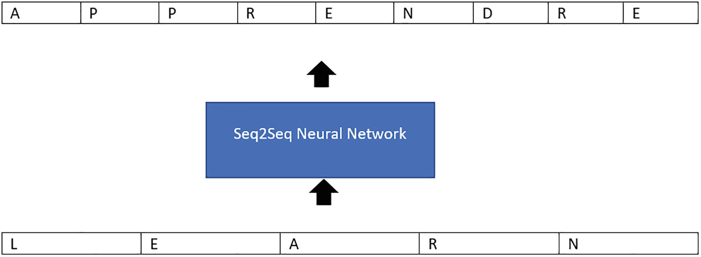
The encoder and decoder are the two components that make up the model as shown in Figure 2-2. The input sequence’s context is saved by the encoder in the form of a vector, which it then transmits to the decoder so that the decoder may construct the output sequence based on the information it contains.
A representation of the sequence-to-sequence order network for the decoder and the encoder which explains the architecture of the translation mask.
Encoder-decoder usage in Seq2Seq networks
Figure 2-2 explains how the encoder and decoder fit into the Seq2Seq architecture for a translation task.
We won’t go into details of the Seq2Seq architecture since the book is mostly about transformers. But to understand the essence of Seq2Seq models, they take a sequence as input and transform it into another sequence.
The Transformer
As was discussed in the beginning of this chapter, there was this great paper called “Attention Is All You Need” in which a new neural architecture called the transformer was proposed. The main highlight of this work was a mechanism called self-attention . One of the idea transformer architecture was to move away from sequential processing where we provided input to the network one at a time. For example, in the case of a sentence, the RNN or LSTM will take one word input at a time from the sentence. This would mean the processing will only be sequential. Transformers intended to change this design by providing the whole sequence as input at one shot to the network and allowing the network to learn one whole sentence at once. This would allow parallel processing to happen and also allow distributing the learnings to other cores or GPUs in parallel.
The transformer architecture ’s main point was to only use self-attention for capturing the dependencies between the words in a sequence and not depend on any of the RNN- or LSTM-based approaches.
Transformers
- 1.
Encoder
- 2.
Decoder
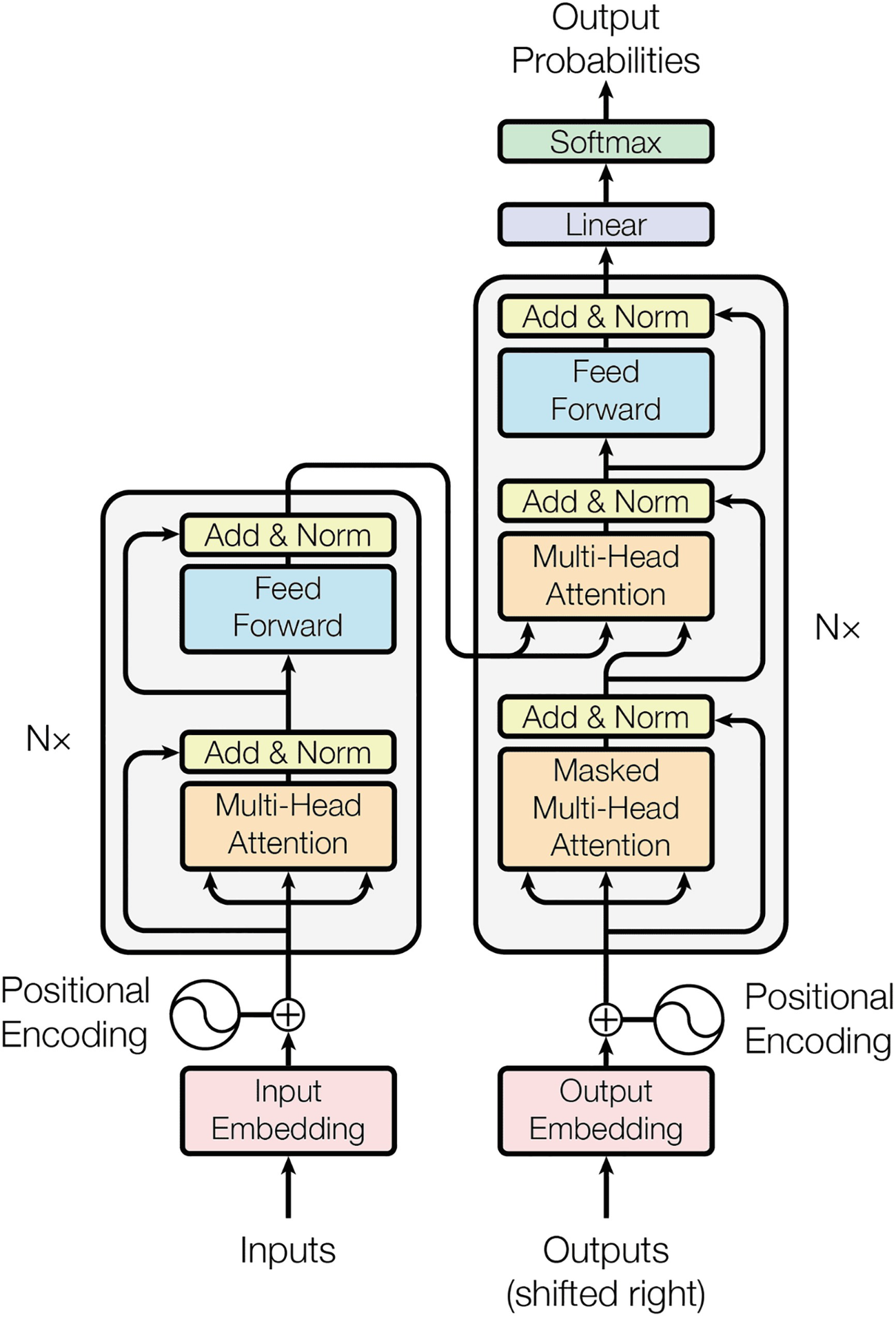
The flowchart represents the inputs and outputs from input embedding and output embedding to output probabilities flowing through positional encoding and N x.
High-level transformer architecture (taken from Vaswani’s “Attention Is All You Need” paper)
Encoder
Let us take a look at the individual layers of the encoder in detail.
Input Embeddings
The first thing that has to be done is to feed input into a layer that does word embedding. One way to think of a word embedding layer is as a lookup table, which allows for the acquisition of a learned vector representation of each word. The learning process in neural networks is based on numbers, which means that each word is associated with a vector that has continuous values to represent that word.
Before applying self-attention, we need to tokenize the words of a sentence into individual tokens.
Tokenize
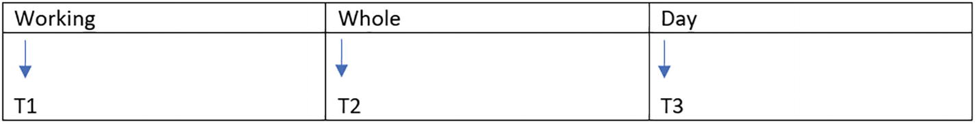
A representation of the tokenization process for a sentence where each word of the sentence is tokenized with a column of working to T 1, whole to T 2, and day to T 3.
Word tokenization in a sentence
Vectorize

A representation of the column of the tokenize and the vectorize which involves the row of Working from T 1 to V 1, Whole from T 2 to V 2, and Day from T 3 to V 3.
Vectorize each token individually to create a mathematical representation of the word
Positional Encoding
It’s an encoding based on the position of a specific word, say, in a sentence.
This encoding is based on which position the text is within a sequence. We need to provide some information about the positions in the input embeddings because the transformer encoder does not have recurrence as recurrent neural networks do. Positional encoding is what is used to accomplish this goal. The authors conceived of a cunning strategy that makes use of the sine and cosine functions.

This equation calculates the positional embeddings of each word so that each word has a positional component alongside the semantic component.
The mathematical specifics of positional encoding are outside the scope of this discussion; however, the fundamentals are as follows.
As demonstrated in Equation 2-1, we pass the word at the odd index via the cosine function and at the even index via the sine function. The output of each word would be a vector that represents the positional encoding of the specific word. We explain this in the following via an example.
Example of Positional Encoding
Take a sequence, say, “Sam loves to walk.”
Here, first we define the values of some parameters:
N: 10000.
K: Position of a word in a sentence starting from 0.
D: Dimension of a sentence. In our case it’s 4.
I: Used for mapping to column index.
Now we calculate the values of the sine and cosine components.
sin(0/10000(0/4))=0 | cos(0/10000(0/4))=1 | sin(0/10000(2/4))=0 | cos(0/10000(2/4))=1 |
sin(1/10000(0/4))=0.8414 | cos(1/10000(0/4))=0.5403 | sin(1/10000(2/4))=0.0099 | cos(1/10000(2/4))=0.999 |
sin(2/10000(0/4))=0.909 | cos(2/10000(0/4))=-0.416 | sin(2/10000(2/4))=0.0199 | cos(2/10000(2/4))=0.9998 |
sin(3/10000(0/4))=0.1411 | cos(3/10000(0/4))=-0.989 | sin(3/10000(2/4))=0.0299 | cos(3/10000(2/4))=0.9995 |
We can see how each word from the sentence “Sam likes to walk” has got a word embedding vector to represent the position of the word in the sentence.
After that, add those vectors to the input embeddings that correspond to those vectors . The intuition behind adding the positional embeddings to the input embeddings is to give each word a small shift in vector space toward the position the word occurs in. So if we think a bit more about it, we can see this leads to semantically similar words that occur in near positions to be represented close by in vector space. Because of this, the network is provided with accurate information regarding the location of each vector. Because of their linear characteristics and the ease with which the model may learn to pay attention to them, the sine and cosine functions were selected together.

A flowchart of encoder components from positional embedding, multi-head attention, add and norm, feed-forward, add and norm to input representations.
Encoder component of the transformer
Multi-headed Attention
The encoder makes use of a particular attention process known as self-attention in its multi-headed attention system . A multi-headed attention is nothing but multiple modules of self-attention capturing different kinds of attentions. As specified earlier in the chapter, self-attention allows us to associate each word in the input with other words in the same sentence.
Let’s go a bit deeper into the self-attention layer.
“Sam had been working whole day so he decided to take some rest”
In the preceding sentence, as humans when the word he is uttered, we automatically connect it to Sam. This simply implies that when we refer to the word he, we need to attend to the word Sam. The mechanism of self-attention allows us to provide a reference to Sam when he is uttered in this sentence. As the model gets trained, it looks at each individual word in the input sequence and tries to look at words it must attend to in order to provide a better embedding for the word. In essence it captures the context better by using the attention mechanism.
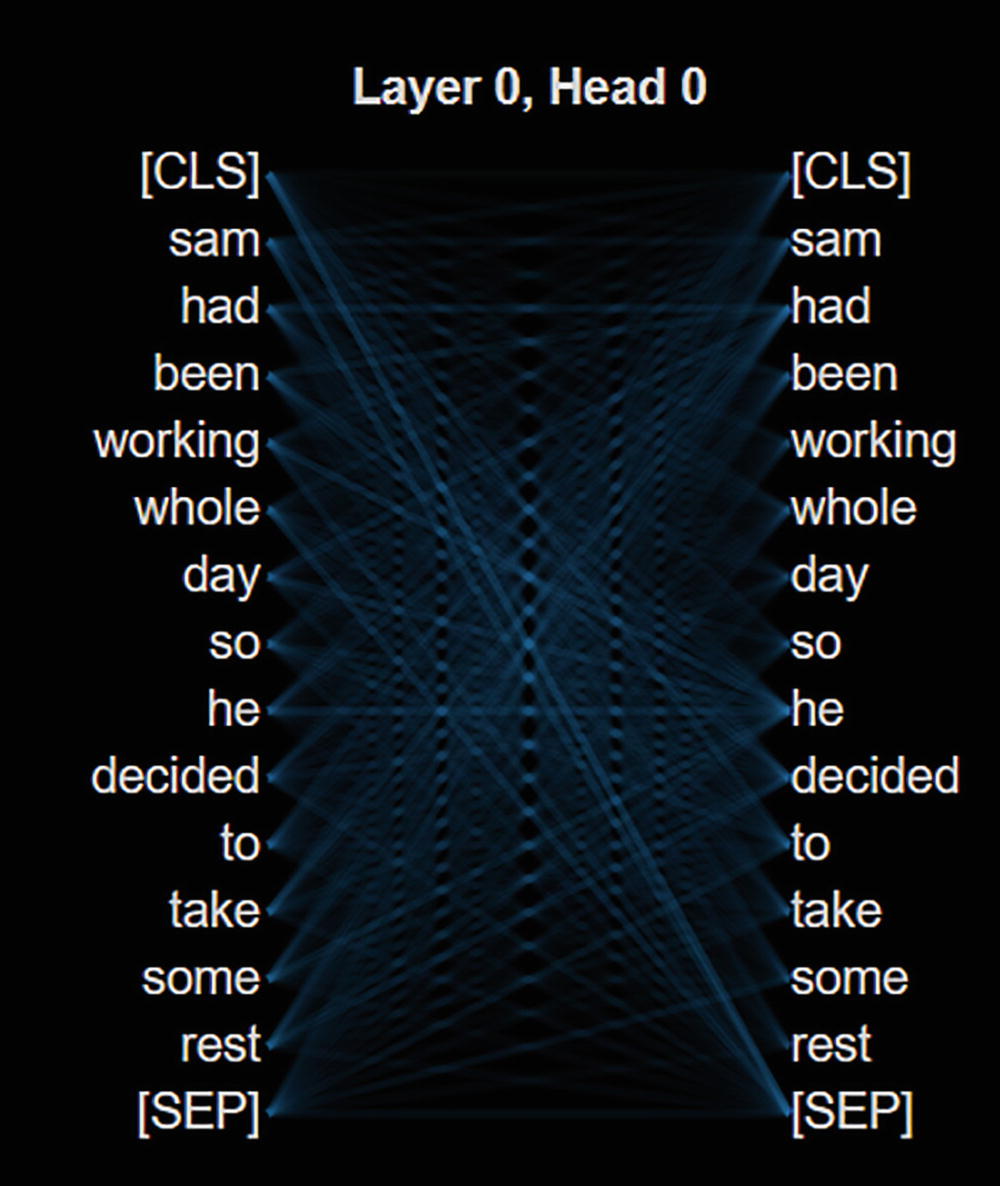
A represents the word he pays attention to the word Sam by using a self-attention technique with layer 0, head 0 involving words like Sam, had, whole, take, etc.
Attention mechanism at work
Next, we take a look into how query, key, and value vectors work.
Query, Key, and Value Vectors
- 1.
Query
- 2.
Key
- 3.
Value
The query, key, and value concept emerged from information retrieval systems. As an example when we search in Google or for that matter any search engine, we provide a query as input. The search engine then finds specific keys in its database or repository that match the query and finally will return the best values back to us as a result.
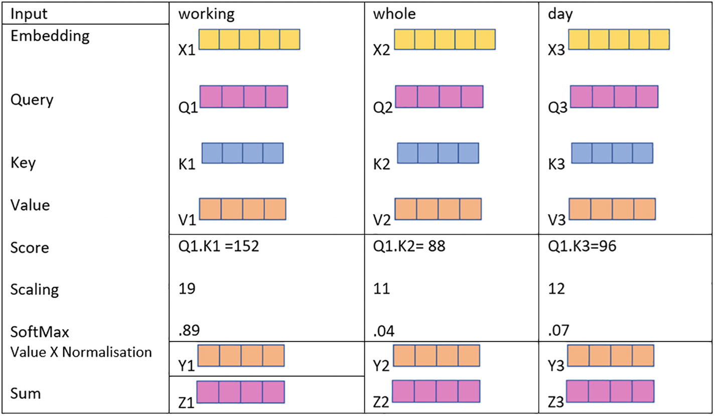
The picture represents the context information by the column of input, working, whole, and day involving embedding, query, key, value, score, scaling, softmax, and sum.
Query, key, and value mechanism at work
Self-Attention
As explained in Figure 2-8, once we have the input vector prepared, we pass it to a self-attention layer, which actually captures the context of the word in its representation by using an attention mechanism.
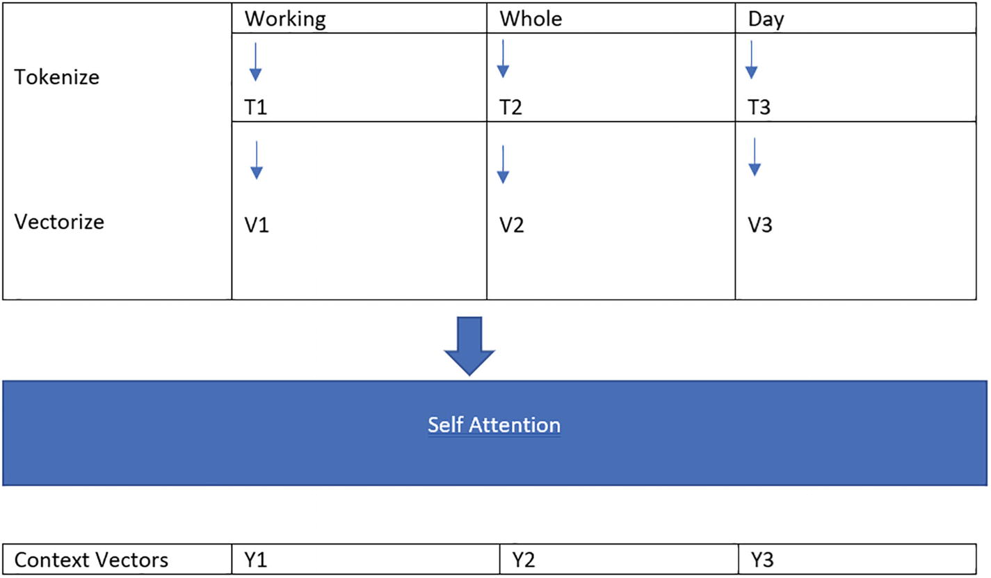
A representation of the context vectors by the column of the tokenize and the vectorize and row of working from t 1 to v 1, whole from t 2 to v 2, and day from t 3 to v 3.
Self-attention mechanism
- 1.
We do a dot product with self and other vectors.
- 2.
We get a score, say, S11,S12,S13 – in this case we have three words in a sentence and we want to capture embedding for V1.
- 3.
This score is then treated as weight and multiplied by V1, V2, and V3.
- 4.
Normalize the score.
- 5.
The sum of the vectors obtained in step 3 is done.
The intuition of the preceding steps is to capture the closeness of words in vector space to each other and then assign weights based on that closeness. Then the neighbor vectors are weighted according to the weight they exercise and added together to give a representation of a word, which takes into account the closeness of words in its neighborhood.
Though this mechanism is simple, there is no learning of weights happening in this. And this is where the mechanism of query and key matrices comes into the picture . The weights in these matrices are what are learned by the network. Each individual word vector does a dot product with the query and key matrix to give a query and key vector.
Following the execution of a linear layer on the query, the key, and the value vector, the production of a score matrix is accomplished by performing a dot product matrix multiplication on the queries and the keys.
The score matrix is used to calculate the relative weight that each word should have in relation to the other words. As a result, every word will be assigned a score, keeping the surrounding contextual words. The higher the score for a specific word, the more it is attended to. This is the process that is used to map the queries onto the keys.
After that, the scores are lowered by having their total divided by the square root of the dimension that contains both the query and the key. This is done in order to make it possible to build gradients that are more stable, as multiplying values can have explosive effects.
After that, you must take the softmax of the scaled score in order to obtain the attention weights, which will provide you with probability values ranging from 0 to 1. When you perform a softmax, the better results are amplified, while the lower levels see a downward adjustment. Because of this, the model is able to have a greater sense of confidence regarding the terms to which they should pay attention.
Multiply the Softmax Output with the Value Vector
After that, you get an output vector by taking the attention weights and multiplying them by your value vector. The higher the softmax scores , the more vital it will be to preserve the values of the words that the model learns. The words with lower scores will be drowned out by those with higher scores. The output of it is then processed by a linear layer after it has been fed into it.
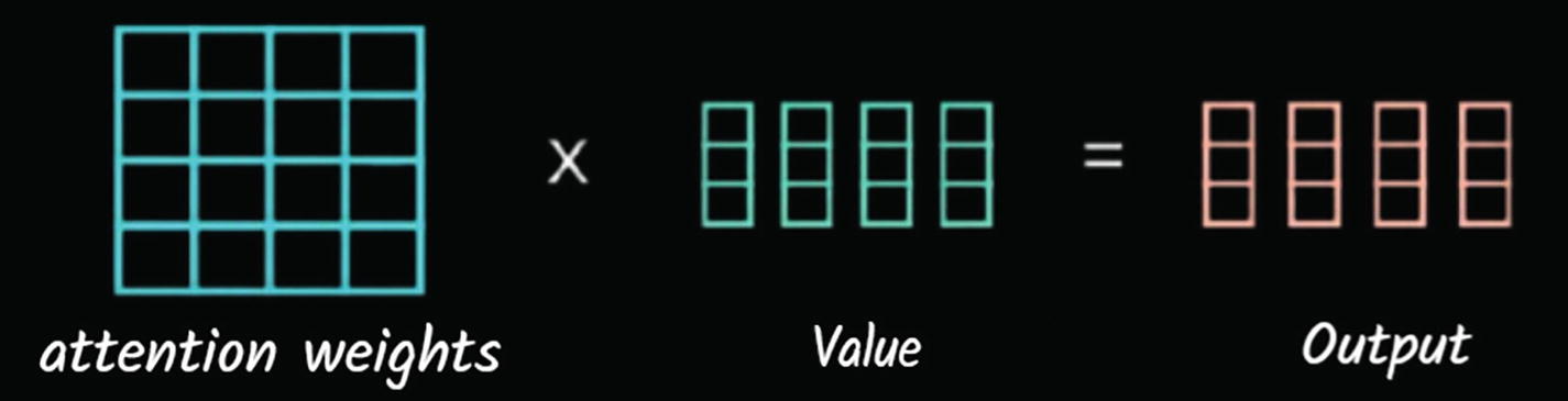
A representation of the mechanism of the attention weights grid multiplied by the value vectors equal to the output which is processed by the linear layer.
Multiply attention weights by the value vectors
Computing Multi-headed Attention
Before applying self-attention , you must first divide the query, the key, and the value into N vectors so that you may do a multi-headed attention computation with this data. After that, each of the split vectors goes through its own particular process of self-attention. The term “head” refers to each individual process of self-attention. Before passing through the last linear layer, the output vectors that are generated by each head are combined into a single vector by means of concatenation. In principle, each head would learn something unique, which would result in the encoder model having a greater capacity for representation.
Multi-headed attention is just self-attention applied multiple times in different ways. The goal is to capture the different contextual representations via these different heads. By using multi-headed attention, the representations we get for a specific word are very rich.
The Residual Connections, Layer Normalization, and Feed-Forward Network
The original positional input embedding is then given the multi-headed attention output vector as an additional component. This type of connection is known as a residual connection. You can think of this step as addition of input (positional encoding in this case) to the output (multi-headed attention output in this case) . After this an operation known as layer normalization is performed on the output of the residual connection. The goal of layer normalization is for improving the performance of training.
Post normalization, the output is passed via a feed-forward network, and then the result of this feed-forward network is normalized with input as the data fed to the feed-forward network.
Because they enable gradients to move directly across the network, the residual connections are beneficial to the network’s training process. The layer normalizations are what are responsible for stabilizing the network, which ultimately leads to a significant cut in the amount of training time required.
This is more or less at a high level how the encoder works. Next, we discuss in brief the decoder component of transformers.
Decoder
- 1.
Multi-headed attention layer
- 2.
Add and norm layers
- 3.
Feed-forward layer
In addition it has a linear layer with a softmax classifier to emit probabilities of an output. This is where the generative part comes into play.
The decoder works by taking the starting tokenized word and then previous outputs if any and combining it with the output of the encoder.
The different aspects involved in the decoding process are explained in the following.
Input Embeddings and Positional Encoding
To a large extent, the beginning of the decoder is identical to the beginning of the encoder. In order to obtain positional embeddings, the input is first placed via an embedding layer and then a positional encoding layer. The positional embeddings are then sent through to the first multi-head attention layer.
First Layer of Multi-headed Attention
This layer, though similar in name to what we used in encoders, is a bit different in functionality . The reason is that the decoder only has access to words that come prior to the current word in the sentence. It’s not supposed to see what word comes next in the sequence.
There needs to be a way for us to avoid computing attention scores for terms in the future. The technique in question is known as masking . By using a lookahead mask, you can restrict the decoder from looking at tokens that are yet to come. The mask is included both before and after the softmax calculation, which takes place after the scores have been scaled. We won’t discuss the mathematical details of the lookahead mask in this book. The basic idea of the mask is to only calculate the attention score for the current word based on previous words and not for future words in the sentence.
Second Layer of Multi-headed Attention
This layer takes the output from the first multi-headed attention layer of the decoder and combines this with the output of the encoder. This will enable the decoder to understand better as to which components of encoder output to attend to. The output of this multi-headed attention layer is passed via a feed-forward network.
Linear Classifier and Final Softmax for Output Probabilities
The output of the previous multi-headed attention layer and feed-forward network is again normalized and passed to a linear layer with a softmax component for emitting the probabilities – as an example, the probability of what could be the next word in a specific sequence of words. This is where the generative aspect of the architecture shines.
Summary
This chapter explained how transformers work. Also it detailed out the power of the attention mechanism that is harnessed by transformers so that they can make more accurate predictions. Similar goals can be pursued by recurrent neural networks, but their limited short-term memory makes progress toward these goals difficult. If you wish to encode a long sequence or produce a long sequence, transformers may be a better option for you. The natural language processing sector is able to accomplish results that have never been seen before as a direct result of the transformer design.
In the next chapter, we look into how transformers work from the point of view of code in more detail. We introduce the huggingface ecosystem, which is one of the major open source repositories for transformer models.