The prior chapter provided us with an introduction to clustering techniques and the use of one such clustering technique, Gaussian Mixture Models. Over the course of this chapter, we will implement a separate technique for multivariate clustering: Connectivity-Based Outlier Factor.
Distance or Density?
There are two key approaches to outlier detection: distance-based approaches and density-based approaches. For univariate anomaly detection, we generally focused on distance-based approaches. As Mehrotra explains, “A large distance from the center of the distribution implies that the probability of observing such a data point is very small. Since there is only a low probability of observing such a point (drawn from that distribution), a data point at a large distance from the center is considered to be an anomaly” (Mehrotra, 97). We started off by implicitly assuming that our univariate datasets fit one cluster, a cluster whose shape might approximate a normal distribution. By Chapter 9, we relaxed that assumption and allowed for multiple clusters using Gaussian Mixture Models. In doing so, we also introduced a density-based approach to detecting outliers.
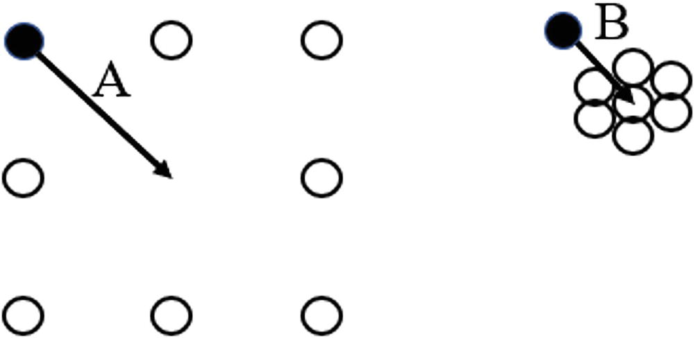
A set of two illustrations of point A and point B comprises 7 small circles. In point, A circles are spread and in point B circles are close.
Vector A is longer than vector B. Therefore, a pure distance-based approach may lead us to believe that point A is more of an outlier than point B
With density-based approaches, we think in terms of neighborhoods, which we can define as a given number of nearest neighbors. We saw this in practice in Chapter 9 with the k-nearest neighbors (knn) algorithm. What differentiates knn from the density-based outlier detection algorithms we will use in subsequent chapters is that knn stops after defining the neighborhood. With density-based outlier detection algorithms, we go one step further: after determining what the neighborhood is for a given point, we then compare the density of that data point vs. its neighbors. If the data point’s density is considerably smaller than that of its nearest neighbors, then the data point is likely to be an anomaly.
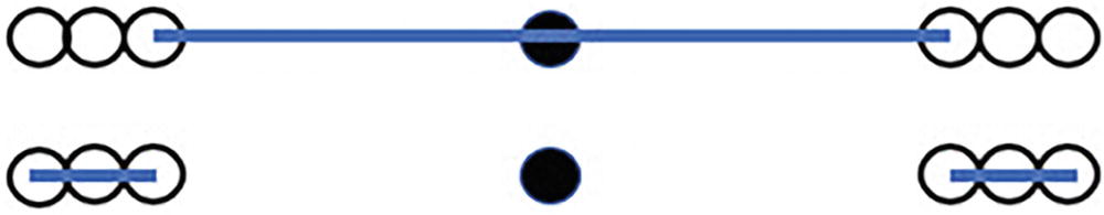
An illustration of the distance of two data points to their two nearest neighbours.
In the top image, we show the distance from our data point (in black) to its two nearest neighbors. In the bottom image, we show the distance from each of those neighbors to their two nearest neighbors
Reviewing the results in Figure 10-2, we can see that the average distance between points is considerably higher for our data point vs. its neighbors. We define the local density of a point as the reciprocal of that average distance between points. Therefore, our data point is in a lower-density area than its neighbors, and this is an indicator of a data point being an outlier.
One important rule that has to hold to make this outcome possible is that the set of neighbors is not reflexive. In other words, if we look at the two nearest neighbors to the black point, neither of them has the black point as one of its two nearest neighbors. As a rule of thumb, the fewer the number of neighbors a data point has that call it a nearest neighbor, the more likely that data point is to be an outlier.
Before we can get to the Connectivity-Based Outlier Factor approach to clustering, we need to understand another algorithm first.
Local Outlier Factor
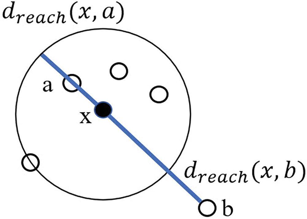
An illustration of a local outlier factor comprises d sub reach x, a and d sub reach x, b.
Calculating reachability distance for data point x with k=5 with respect to two other data points a and b. Note that the neighborhood size includes data point x
We then calculate the distance from x to each point, taking the larger of the actual distance or the distance to the kth point as dreach. For example, point a lies within the boundaries of our circle, and so we use the distance to the kth point to define the reachability distance from x to a. Point b, meanwhile, lies beyond our kth point, and so we use the actual distance from x to b as the reachability distance from x to b. After performing this operation for each pairing of data points in our extended neighborhood, we can calculate the average reachability distance for x by summing up all of the reachability distances from x to various points and dividing by the number of points in the cluster minus one (i.e., the denominator will not include data point x itself).
The average reachability distance gives us an idea of how far we need to travel in order to find similar data points. If we take the reciprocal of this, we now calculate the reachability density of a point: How packed-together are other data points near our point x?
Finally, we define the Local Outlier Factor as a ratio of the local reachability densities of all other data points vs. the local reachability density of point x. A relatively high value for this measure means that there tends to be a larger distance between data point x and its neighbors compared to other data points in the cluster. This result comports with one an intuitive understanding of outliers: data points that are far removed from others are more likely to be outliers than ones packed closely together. Once we have the LOF per data point, we can use that score to determine whether a particular data point is an outlier. One way we could do this is to take the top few percent of values and declare those data points as outliers. Alternatively, we could compare the largest scores and use techniques like MAD to see if there is a significant enough spread from the median to declare any given point a likely outlier.
Connectivity-Based Outlier Factor
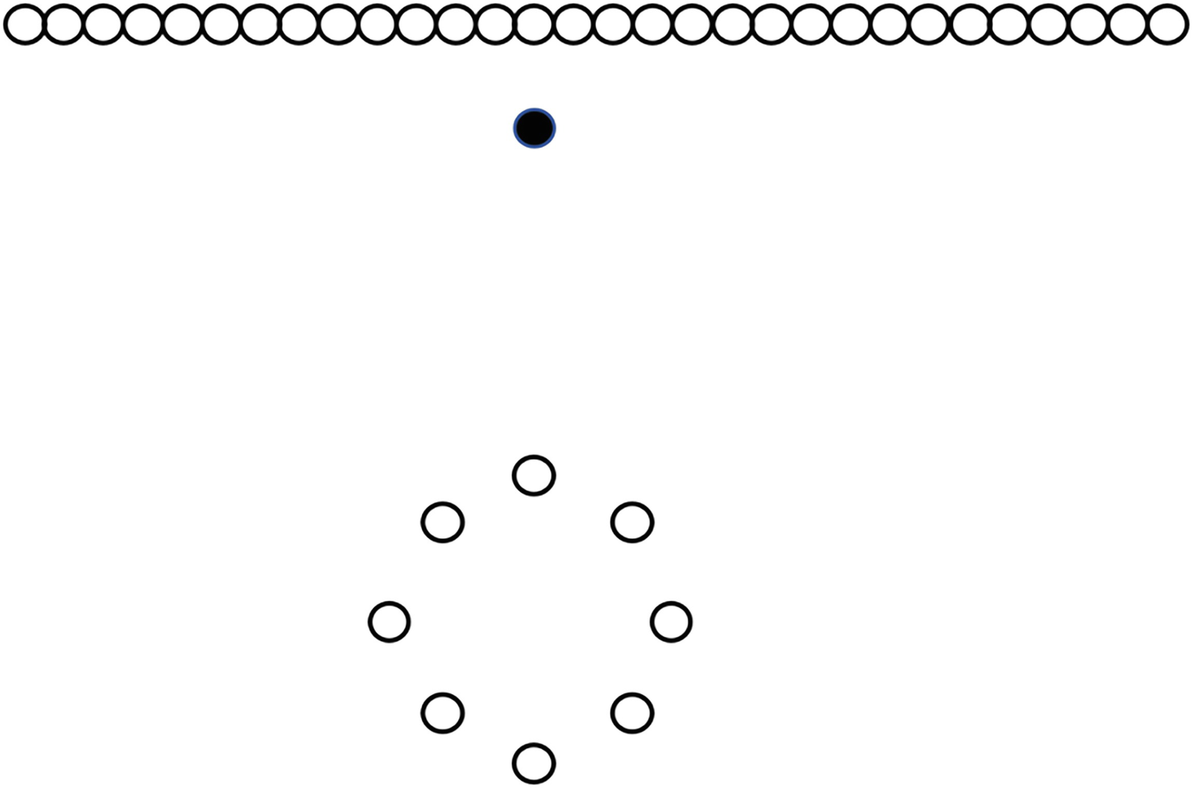
An illustration of a local outlier factor highlights a mass of points at the top and the second cluster of points with some separation between them.
Any value of k that allows LOF to declare the highlighted point as an outlier will also declare all points in the circle as outliers
Here, we can see the outlier, which I have marked as a black dot for the sake of clarity. Note further that there is really only one outlier in this figure: we have a mass of points at the top of the image and a second cluster of points with some separation between them. Using the LOF algorithm, however, we run into a problem: in order to detect the marked point as an outlier, we would also classify all of the points in the circle as outliers because of the difference in distances between elements in the two clusters.
Connectivity-Based Outlier Factor (COF) is another density-based approach to clustering, one that attempts to resolve these sorts of problems with LOF. It does so by adding to density an idea called isolativity: the degree to which an object is connected to other objects. The points making up the circle are connected to one another, just as the points in the line at the top of the figure are connected to one another. The marked point, however, does not fit either of the established patterns—it is isolated from those patterns and is therefore more likely to be an outlier than a point that is connected in a pattern.
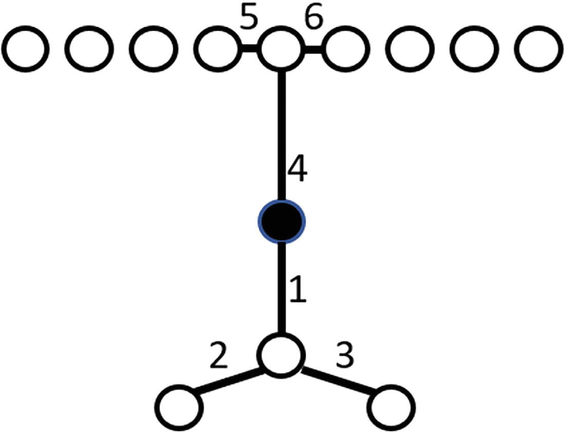
An illustration of a connectivity-based outlier factor highlights the market point with six connections between seven points.
The six connections for the marked data point. Note that edges are enumerated sequentially in order of the shortest path from the already-connected chain to the next free point
Once we have these connections, we perform a weighted calculation, emphasizing the “earlier” (numerically lower) connections more than the “later” (numerically higher). This provides us the Connectivity-Based Outlier Factor (COF) value. Data points with higher COF values are more likely to be outliers than data points with lower COF values. This allows us to sort data points by COF value in descending order and find the biggest outliers, something that is particularly handy if the base algorithm returns more outliers than our maximum fraction of anomalies parameter allows.
The math for calculating COF is available in Tang et al., but because we are going to use the Python Outlier Detection (PyOD) library to calculate COF, we will not include it here. Instead, we will move on to implementation.
Introducing Multivariate Support
The code for multivariate anomaly detection will necessarily look somewhat different from univariate anomaly detection—after all, the data structure for multivariate anomaly detection includes a key and list of values vs. a key and a single value for univariate anomaly detection. Even so, there will be considerable overlap in the groundwork code.
Laying the Groundwork
Offering multivariate outlier detection to outside callers
Based on this definition, we know that we will need a detect_multivariate_statistical() function in our code base. We will also want helper functions like run_tests() and determine_outliers(), similar to our univariate example.
A function to detect outliers in multivariate data. Certain diagnostic functionality has been removed from this listing for the sake of brevity, but it is available in the accompanying repository.
Encoding string data
Even though we do include an encoding function, it is important to note that the way we are encoding is easy but not necessarily a good practice. The reason is that our encoder is ordinal and does not include any measurement of string “nearness,” either in terms of how many letters apart two words are or how similar (or dissimilar) the meanings of two words are. As an example, the word “cat” might have an ordinal value of 1 but “cats” a value of 900. Our transformation is simple and likely will not work well on text-heavy datasets. The intent here is to provide an easy method for working with a mostly numeric dataset that happens to have one or two categorical string features, rather than analyzing the textual content of features and discerning meaning from them. It is possible to create a more sophisticated encoder that does this, but that is an exercise for another book on natural language processing.
Implementing COF
Implementing the check for Connectivity-Based Outlier Factor
The run_tests() function is very similar to its univariate counterpart, saving the interesting code for check_cof(). This latter function accepts our DataFrame as well as the max fraction of anomalies and desired number of neighbors. It first creates an array out of all columns except key and vals, as the COF function requires inputs be shaped as an array rather than a DataFrame. After creating a classifier function using COF(), the function fits the classifier to our input array. We use the corresponding labels_ attribute to see if COF considers a particular data point as anomalous and decision_scores_ to gain an idea of how much of an outlier a given data point is. The contamination factor, which we capture as clf.contamination, is an optional input that defaults to 0.1 and represents the proportion of outliers in the dataset. This is similar to what we call the max fraction of anomalies in our engine, except that contamination factor requires that we mark a certain percentage of results as outliers, no matter how high or low the decision score is. If we set the contamination factor to 0.5, half of our data points will be marked as outliers, even if every data point is tightly clustered together and a human would not recognize any data points as anomalies. The threshold_ output provides the cutoff point for what COF labels as an outlier.
The outlier determination function for multivariate outlier detection
We start by calculating the sensitivity score. Because our anomaly score range may be quite different from 0 to 1, we adjust the sensitivity_score range to run from 0 to the second-largest anomaly score, dealing with cases in which one extreme outlier dominates everything else. After doing that, the calculations are the same as the univariate scenario. An important note here is that, unlike the univariate scenario, we could always get back a number of anomalies equal to max_fraction_anomalies * number of data points when sensitivity score is set to 100. COF does not have any in-built rules around whether a particular point is an outlier or not, making our selection of max fraction of anomalies and sensitivity score even more important than in the univariate scenario. That said, values closer to 1.0 are less likely to be outliers, and choosing some minimum threshold will reduce the number of spurious outliers. 1.35 is an arbitrary choice but one that is intended to prevent an outcome in which a dataset with no actual anomalies triggers a large number of reported outliers.
Test and Website Updates
This new technique brings with it a new set of tests, as well as some challenges we will need to face regarding visualization of multivariate data. Let’s start first with unit test changes, move on to integration tests, and end with website updates.
Unit Test Updates
Encode strings as ordinal values
Reviewing the aforementioned, there are two string columns per array. The encoding function correctly sees this and dutifully encodes the strings in the second and fourth columns of the array.
Aside from this, there are several other functions intended to test COF’s outputs and how sensitivity score and max fraction of anomalies combine to affect outcomes. There are three datasets that we will use in the tests. The first is sample_input, which contains an artificially generated set of data spanning four columns. It includes a fairly wide range of values, making it difficult to determine a priori whether there are any outliers. The second dataset is sample_input_one_outlier, which includes dozens of extremely similar rows, differing by no more than ~1%, as well as one radically different row. Finally, sample_input_no_outliers is the prior dataset minus the one outlier.
The minimum anomaly score check in determine_outliers() is critical for scenarios like sample_input_no_outliers. If we have no minimum threshold and set maximum fraction of anomalies to 1.0, we would need to drop the sensitivity score down to 8 in order to have fewer than ten outliers returned. With no cutoff and very close data points, instead of having no outliers, everything becomes an outlier.
Integration Test Updates
Along with new unit tests, we also need new integration tests to handle multivariate data. These tests are in the Chapter 10 Postman collection and handle fairly basic scenarios ranging from zero to three outliers in a small, 15-record sample. The most interesting of these tests is Ch10 – Multivariate – Debug – Three Outliers, 2S1L – Two Recorded. This test includes three outliers at three different orders of magnitude. The first outlier has an anomaly score over 100, the second has a score of 34, and the third has a score of 5.8. All three are legitimate outliers, but unless we set the sensitivity score to 83 or higher, we only capture the two larger outliers because the largest outlier “sets the curve” and makes it harder for us to find smaller outliers. This points at a flaw in our solution, one we aim to rectify over the next two chapters by introducing additional algorithms and forming a new type of ensemble.
Website Updates
The definition for the process() function
Creating a visual to expose multivariate outlier results
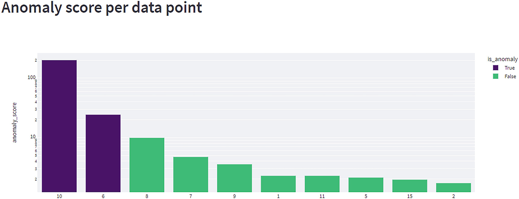
A bar graph plots anomaly score versus values. Values are estimated. True (10, 100 to the power 2), (6, 10 to the power 2.5). False (8, 10), and more.
The outcome of a multivariate anomaly detection test. This shows the key as the X axis and the anomaly score on a logarithmic scale as the Y axis
After that, we display a table of all keys and values. Finally, if the user wishes to see debug information, we can see debug weights, tests run, and test diagnostics below the table.
Conclusion
In this chapter, we looked at one useful algorithm for multivariate outlier detection: Connectivity-Based Outlier Factor (COF). This is a good first algorithm to look at because it tends to be quite effective. As we saw in the test cases, though, understanding the appropriate cutoffs can be a challenge. In the next chapter, we will introduce another, complementary technique to COF and see how to combine the two together in an ensemble to reduce some of the challenge of picking appropriate inputs and cutoff values.