Discovering the Neighborhood

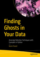
An important difference between LOCI and other density-based approaches like LOF or COF is that LOCI does not ask for an explicit number of neighbors in a neighborhood. Instead, it takes a measure called alpha (α), which represents neighborhood size, with 0 < α < 1. The default value for α is 0.5; Papadimitriou et al. chose this value for their experiments (Papadimitriou et al., 5), and we will stick with this value.

Along with α, we need a variable r, which represents the distance of our sampling neighborhood: the set of points we will use against which to compare a given point. Specifically, we determine if that data point is an outlier based on the number of neighbors within a bounded circle measuring α * r, otherwise known as the counting neighborhood. Figure 11-1 provides a visual example of this.

A Venn diagram of 2 sets. It has 2 concentric sets with a radius of r and the inner set has a radius of a r from the point P 1.

Within our counting neighborhood α * r, we count the number of data points that exist, giving us an idea of how densely packed data points are near our point of interest. Then, to gain an understanding of how that compares to other points, we repeat the process for each point inside our sampling neighborhood. Figure 11-2 fills in additional detail, introducing two additional points: p₂ and p₃. Because these two points exist inside p₁’s sampling neighborhood, we use these two points to compare against p₁. The results we come up with are that p₁ has one data point in its counting neighborhood, p₂ has three, and p₃ has five, noting that counts are inclusive of the tested data point.

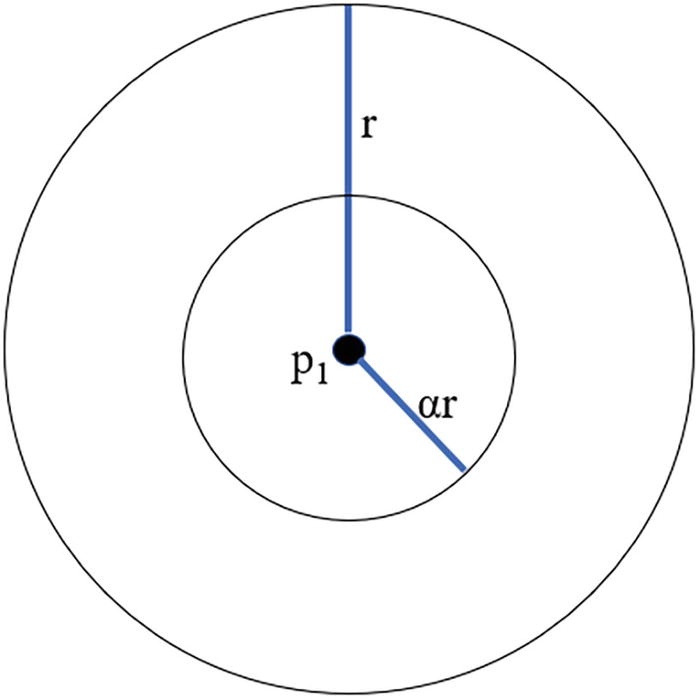
A Venn diagram of 11 sets. It has 2 concentric sets with a radius of r and the inner set has a radius of A R from the point P 1. The intersecting areas of sets on the top right and bottom left are labelled P 2 and P 3, respectively.

From the image in Figure 11-2, we can determine two important criteria. The first is the number of data points inside the counting neighborhood, which we can represent as n(p_i, αr). This comes out to 1 for p₁, 3 for p₂, and 5 for p₃, respectively.

The second criterion we can determine is the mean of αr-neighbors within a given sampling neighborhood, which we can represent as In this case, the mean is 3.

With these two criteria, we can calculate the Multi-granularity Deviation Factor.

Multi-granularity Deviation Factor (MDEF)

The Multi-granularity Deviation Factor (MDEF) is defined using the formula in Listing 11-1.

r

Listing 11-1

The formula for Multi-granularity Deviation Facto

In other words, we take the size of our counting neighborhood and compare it to other counting neighborhoods in our sampling area. In our example, p₁ has an MDEF of 2/3, p₂ an MDEF of 0, and p₃ an MDEF of -2/3.

The actual outlier detection process takes the standard deviation of counting neighborhood sizes over the sampling neighborhood, as we see in Listing 11-2.

F

Listing 11-2

Calculating the standard deviation of MDE

Once we have the standard deviation of MDEF, we get to the other input parameter aside from α: k, which represents the number of standard deviations from MDEF before we consider a data point an outlier. To this, we can apply our rule of thumb from Part I of the book: three standard deviations from the mean indicate a data point as an outlier. Papadimitriou et al. describe the formal logic behind this calculation and indicate that when k=3, we can expect fewer than 1% of data points to trigger that threshold if the set of neighborhood sizes follows a normal distribution (Papadimitriou et al., 5).

Now that we have some understanding of how the LOCI algorithm works, we can incorporate it into our multivariate outlier detection model.

Ensemble Types

There are two main classes of ensemble: independent ensembles and sequential ensembles. In Part II, we implemented a form of independent ensemble using weighted shares. The main idea behind an independent ensemble is that we run each test separately, generate each output separately, and combine results at the end. Typically, we return a data point as an anomaly if all—or at least enough—of the tests agree. We can weigh those tests differently based on the quality of different tests. We may, for example, reduce the weight of noisy tests relative to their less error-prone counterparts.

Sequential ensembles, by contrast, stack models like a sieve. The idea here is that the output of one model serves as the input for the next model. In practice, we tend to have the most sensitive (and often noisiest) model go first, giving us a provisional set of outliers. Then, for each additional algorithm, we need only to perform the next set of calculations on the remaining set of outliers—if prior, noisier models think a data point is an inlier, we can accept it as such and save the computational effort. The main benefit to a sequential ensemble is that it can quickly narrow down very large datasets, making it a great approach for enormous datasets. If you are dealing with tens or hundreds of millions of records, a noisy approach should still filter out 90–95% of the data points out of the gate, leaving us with a much smaller fraction for the less noisy but more computationally expensive methods.

The major downside to sequential ensembles is that they tend to require more programming effort, as out-of-the-box implementations of algorithms in libraries like PyOD assume you will care about the entire dataset rather than a small selection of data points. In an effort to minimize complexity, we will again use an independent ensemble for multivariate analysis. This is an area, however, in which it can make sense to invest in developing a sequential ensemble, as the implementations of COF and (especially) LOCI we will use can be time-intensive even for small datasets.

Before we bring LOCI into the mix, it is worth taking a return trip to COF.

COF Combinations

By the end of Chapter 10, we created a multivariate outlier detection system using COF as the centerpiece. COF is a great algorithm, but it does require that callers choose the size of the neighborhood and the cutoff point for what constitutes an outlier. Our implementation partially handled the second item by setting a minimum boundary of 1.35 but left the choice of number of neighbors entirely to the caller. This is a reasonable solution, but we can do better: we can try COF with different combinations of neighbor counts (within reason) and combine the results of each test together as an ensemble. To do so, we need the combination module in PyOD.

In this function, we use the range() function to generate a series of nearest neighbor counts to try, starting with the user-defined total (or its default of 10) and moving up by increments of 5 to the lesser of 100 plus the original nearest neighbor count or five less than the number of records in the dataset. For example, with 1000 data points and a starting nearest neighbor count of 10, we will get back a total of 21 values, ranging from 10 to 105. By contrast, if we have 20 data points and a starting nearest neighbor count of 4, we will get back three values: 4, 9, and 14. We then build out two-dimensional arrays named labels_cof and scores_cof to store the results of each test. For each value in the nearest neighbor range, we call check_cof(), sending in the column array, max fraction of anomalies, and number of neighbors, storing the results in our array.

After we have taken care of running COF the prescribed number of times, we need to combine the results somehow. PyOD includes several mechanisms for determining the final value for an outlier score or label. Three options are intuitive: median(), average() (which performs the mean), and maximization(). Another useful option is majority_vote(), which we use for determining our label values. Two other interesting options are Average of Maximum (AOM) and Maximum of Average (MOA). AOM and MOA require a number of buckets, which defaults to 5. Then, we randomly allocate results to each of the buckets. For AOM, we find the maximum value in each bucket and calculate the mean across each of those bucket maxima. For MOA, we calculate the mean of each bucket and return the maximum of those values. With both measures, we can smooth out scores across runs for a given data point. For example, if a COF score for a given data point is normally in the 1.1–1.3 range but a single run results in a COF of 7, this can affect our average() and maximization() functions but will have a very small effect on median(), MOA, and AOM. There can be some benefit to using one of AOM or MOA to calculate our response, but median will work well enough and also ensures that we do not need to consider how many buckets we would need for any given dataset. For that reason, we will use the median to calculate our anomaly score.

By incorporating a variety of tests covering different numbers of neighbors, we have a more robust calculation of COF, and we can also remove an unnecessary decision from our users in how many neighbors to choose. We are now ready to incorporate LOCI into the mix.

Incorporating LOCI

The first change we see determines whether to run LOCI. As of the time of writing, the implementation of LOCI in PyOD is very inefficient and can struggle with larger datasets. For this reason, if our dataset is too large, we will not run LOCI and will depend on the more efficient implementation of COF. Assuming we do run LOCI, we call the check_loci() function. Note that we do not pass in values of α or k; we leave those at their defaults of 0.5 and 3, respectively. The LOCI algorithm also determines the value of r for us automatically, so we do not need to pass anything in for that parameter. What we get back from the check function includes an array of scores, one outlier score per data point. The result of the median(scores_cof) function call is also an array of scores, containing the median data score per data point across all of our COF tests. We simply add these two arrays together, giving us a combined score with no weighting factor. The intuition here is that our minimum threshold for COF is 1.35 and our threshold for LOCI is 3. We expect both values to be fairly close to one another for inliers and near-outliers, so by adding them together, we let a very strong decision by one model out-vote a tepid response from the other. For example, suppose LOCI returns a score of 2.8, which is close but not quite an outlier. If COF returns a score of 20, well above the 1.35 minimum threshold, the strength of COF’s conviction outweighs LOCI’s lukewarm judgement.

We begin the function by calculating the sensitivity threshold, which will be 1.35 if we only ran COF and 4.35 if we ran both COF and LOCI. After that, we calculate the sensitivity score based on the second-largest data point, just as we did in Chapter 10. Then, we determine whether we need to use the sensitivity score or max fraction of anomalies to act as our cutoff, just as we did in Chapter 10. Finally, the return statement creates a new anomaly_score column based on whether a data point clears the larger of our sensitivity score and our sensitivity threshold. One final difference in this function is that we return diagnostic data relating to score calculations, allowing a user to diagnose issues.

Unit Test Updates

There are two changes of note with respect to unit tests. The first is that by running multiple iterations of COF and incorporating LOCI, the number of outliers becomes rather stable: shifts in the sensitivity score and max fraction of anomalies have very little impact until you get to the extremes. On the whole, this is an interesting outcome for us as it means end users should not need to worry about picking the “right” sensitivity score or max fraction of anomalies. The key downside, however, is the loss of control for more advanced users. In the sample input provided with the multivariate test cases, we see five outliers with a sensitivity score of 5. Trying again with a sensitivity score of 25, the number of outliers jumps to eight, and it stays at eight the rest of the way to a sensitivity score of 100. If users anticipate smooth (or at least regular) increases in the number of outliers based on the sensitivity score, they might be confused by this result.

The other change of note comes from the fact that LOCI is more sensitive than COF, at least on our test datasets. For example, the sample inputs with no outliers and one outlier both contain a record whose first input is 87.9 and whose third input is 6180.90844, both of which represent “extreme” values. 87.9 happens to be the largest value we see in the first input and 6180.90844 the smallest value we see in the third, but both are well within 1% of their respective medians. LOCI is capable of spotting this minute difference and flags the data point as an unexpected outlier. To ensure that the tests return the appropriate number of outliers, changing the third value to its median value of 6185.90844 was sufficient to resolve the issue. This level of sensitivity is something to watch out for when using algorithms like COF and LOCI, especially given the first insight around the relative lack of user-controllable sensitivity adjustments.

Website Updates

The first column of our debug menu shows the set of tests run as well as diagnostic information. This diagnostic information includes the number of records in the dataset; the number of neighbors, contamination score, and threshold value for each run of COF; and the LOCI threshold. The second column shows outlier determinants, including our sensitivity threshold and the work we do to calculate sensitivity score. Figure 11-3 shows an example of this using the pre-created sample dataset. Below these two columns, we can see the full debug details as well.

An algorithm for pre-created sample dataset. It has 2 columns labeled tests run and outlier determinants.