Averages

Perhaps the simplest statistic is the average, or mean, or for the mathematically minded, the expectation of a set of numbers. Commonly, when we talk about the average for a dataset, we are talking about the central tendency of the data, the value that “balances” the data. We show how to calculate these by hand in the next section.

We intentionally do not include code for this section, as one of Eric’s professors at the University of Nebraska–Lincoln, Dave Logan, would say, “The details of most calculations should be done once in everyone’s life, but not twice.” We will show you how to use Python and R to calculate these later in this appendix.

To work through this exercise, let’s explore passing plays again, as shown in Chapter 1. This time, you will look at a quarterback’s air_yards and study its properties in an attempt to understand his and his team’s approach to the passing game. We use data from a 2020 game between Richard’s favorite team, the Green Bay Packers, and one of their division rivals, the Detroit Lions, and only then look at plays that have an air_yards reading by Detroit over the middle of the field. “Filtering and Selecting Columns” shows how to obtain and filter this data. Looking at a small set of data will allow you to easily do hand calculations.

First, calculate a mean by hand. The air yards are 5, –1, 5, 8, 5, 6, 1, 0, 16, and 17. To calculate the mean, first sum (or add up) the numbers:

5 + –1 + 5 + 8 + 6 + 5 + 6 + 1 + 0 + 16 + 17 = 68

Next, divide by the total number of plays with air yards:

This allows you to estimate the mean air yards to the middle of the field to be 6.2 yards for Detroit during its first game against Green Bay in 2020. Also, we rounded the output to be 6.2. We need to round because the decimal of the resulting mean does not end and we really need to know only the first digit after the decimal, since the data is in integers. More formally, this is known as the number of significant digits or figures.

Another way to estimate the “center” of a data set is to examine the median. The median is simply the middle number, or the value of the average individual (rather than the average value). To calculate the median, write the numbers in order from smallest to largest and then find the middle number, or the average of the two middle numbers if you have an even number of values.

The last common method to estimate an average number is to examine the mode. The mode is the most common value in the dataset. To calculate the mode, we need to create a table with counts and air yards, such as Table B-1.

With this example, 5 is the mode because three observations provide a reading of 5 air yards. Data can be multimodal (that is to say, have multiple modes). For example, if two outcomes have the same number of occurrences, a bimodal outcome occurred.

Each central tendency measure has its pluses and minuses. The mean of a set of numbers depends heavily on outliers (see “Boxplots” for a formal definition of outliers). If 2022 NFL MVP Patrick Mahomes, who at the time of this writing makes about $45 million annually, walks over to a set of nine practice squad players (each making $207,000 annually as of 2022), the average salary of the group is about $4.5 million per player, which doesn’t accurately represent anything about that group. The median and mode of this dataset doesn’t change at all ($207,000) with the inclusion of Mahomes, as the middle player scoots over half of a spot, and the group with the highest reading is the practice squad salary. That being said, much of the theoretical mathematics that has been built works a lot better with the mean, and discarding data points because they are outside the confines of the middle of the data set is not great practice, either. Thus, as with everything, the answer to which one you should use is “it depends.”

Finally, other kinds of means exist, but they do not appear in this book. For example, in sports betting (or financial investing in general), one will often care about the geometric mean of a dataset rather than the arithmetic mean (which we’ve computed previously). The geometric mean is simply computed by multiplying all the numbers in the dataset together and then taking the root corresponding to the number of elements in the dataset. The reason this is preferable in betting or financial markets is clear: numbers grow (or decline) exponentially in this case rather than additively.

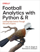
Let’s examine these three measures of central tendency for air yards for all pass locations for both teams from the first game between Green Bay and Detroit in 2020 in Figure B-1. This subset of the data is more interesting to examine but would have been harder to examine by hand.

Figure B-1. Comparing different types of averages, also known as the central tendency of the data

First, notice that the line, labeled mean (blue online), is to the right of the median (red online). This means the data is skewed or has outliers to the right. Second, the median is the same as the mode in this example, so their lines overlap. Most people, including us, usually refer to the mean as the average.

So, what does this tell us about Detroit’s passing in this game? First, the difference between mean and median shows that many pass plays are short, with the exception of a few long passes. This histogram shows us the “shape” of the data and the story it tells us about the game, which are probably better than simple summary statistics. This doesn’t necessarily scale up with the size of the data, but it shows why it’s always good to plot your data when you start and the reason we covered plotting as part of exploratory data analysis (EDA) in Chapter 2.

Variability and Distribution

The previous section dealt with central tendency. Many situations, however, require you to know about the variability in the data. The easiest way to examine the variability in the data is the range, which is the distance between the smallest (minimum, or min) and biggest number (maximum, or max) in the data. For data shown in Table B-1, the min is –1 and the max is 17, so the range is 17 – –1 = 17 + 1 = 18.

Another method to examine the range and distribution of a dataset is to examine the quantiles. These focus on specific parts of the distribution, and their use can avoid the strength of severe outliers. The $n$th quantile is the data point where n% percent of the data lies underneath that data point. You’ve already seen one of these before, as the 50th quantile is the same thing as the median. “Boxplots” covered quantiles (specifically within the context of boxplots). The 25th, 50th, and 75th quantiles are commonly referred to as quartiles, and the difference between the first quartile and the third is the interquartile range (IQR).

Recall that boxplots show us where the middle 50% of the data occurs. Sometimes, other types of quantiles may be used as well. The benefit of quantiles are that they are estimated end points other than the central tenancy. For example, the mean or median allows you to examine how well average players do, but a quantile allows you to examine how well the best players do (for example, what does a player need in order to be better than 95% of other players?).

The most common method for examining the variability in a dataset is to look at the variance and its square root, the standard deviation. Broadly, the variance is the average squared deviation between the data points and the mean. The square is used so that the distance between each data point and the mean is counted as positive—so variability beneath and above the mean don’t “cancel out.” Using the Detroit Lions air yards example, you can do this calculation by hand with the numbers supplied in Table B-2. We include a mean column in case you are doing this calculation in a spreadsheet such as Excel and to also help you see where the numbers come from.

After you create this table, you then take the sum of the difference squared column, which is 4,177. You divide that result by 76 because this is the number of observations minus 1. The reason to subtract 1 from the denominator has to do with the number of degrees of freedom at dataset has—the amount of data necessary to have a unique answer to a mathematical question.

Calculating $\frac{4,177}{(77-1)}$ gives the variance, 54.96. The units for variance with this example would be yards $\times$ yards, or yards². This does not relate that well to the central tendency of the data, so we take the square root to get the standard deviation: 7.41 yards, which is now in the units of the original data. All statistical software can calculate this value for you, and comparing variances and standard deviations across various datasets helps you compare the variability of multiple sources of data easily and in a way that scales up. Often, you will divide the standard deviation by the mean to get the coefficient of variation, which is a unit-less measure of variability that takes into account the size of data points. This might be important when comparing, say, passing yards per play to kickoff returns per play. One is on the order of 10, and the other is on the order of 20, and the variability understandably scales with that.

Uncertainty Around Estimates

When people give you predictions or summaries, a reasonable question is how much certainty exists around the prediction or summary? You can show uncertainty around the mean using the standard error of the mean, often abbreviated as SEM, or simply SE, for standard error. More informatively, you can estimate confidence intervals (CIs). The most commonly used CI is 95% because of historical convention from statistics. The CI will contain the true or correct estimate 95% of the time if we repeat our observation process many, many times. If you accept this probability view of the world, you will know your CIs will include the mean 95% of the time, but you just won’t know which 95% of the time.

The standard error is not the same thing as the standard deviation, but they are related. The former is trying to find the variability in the estimate of the population’s mean, while the latter is trying to find the variability in the population itself. To compute the standard error from the standard deviation, you simply divide the standard deviation by the square root of the sample size. Thus, as the sample size n grows, your estimate for the population’s mean becomes tighter, and the standard error decreases, while the variability in the population is fixed the whole time.

To calculate upper and lower bound of a confidence interval, use the empirical rule as a guide. The empirical says that, approximately 68% of the data lands within one standard deviation of the data, 95% within two standard deviations, and 99.7% within three. These values change with different distributions, and work best with a normal distribution (also known as a bell curve), but are pretty stable with respect to situation. The actual value for a 95% CI is 1.96.

Continuing with the previous example, calculate the standard error: $7.41/\sqrt{77}=0.84$. Thus, you can write the mean as 8.03 ± 0.84(SE), or with the 95% CI as 8.03 (95% CI 6.38 to 9.68), which is calculated by 8.03 ± 0.84 × 1.96 = 1.64.

Based on statistical convention, you can compare 95% CIs to examine whether estimates differ. For example, the estimate of 8.03 (6.38 to 9.68 95% CI) differs from 0 because the 95% CI does not include 0. Thus, you can say that the air yards by the Detroit Lions in week 2 of 2020 differ from 0 when accounting for statistical uncertainty. If you were comparing two estimated means, you could compare both 95% CIs. If the CIs did not overlap, you can say the means are statistically different.

Chapter 3 and other chapters cover more about statistical inferences. Chapter 5 also covers more about methods for estimating variances and CIs. Now, enough about theory and hand calculations; let’s see how to estimate these values in Python and R.