Exploratory Data Analysis

Prior to running a simple linear regression, it’s always good to plot the data as a part of the modeling process, using the exploratory data analysis (EDA) skills you learned about in Chapter 2. You will do this using seaborn in Python or ggplot2 in R. Before you calculate the RYOE, you need to load and wrangle the data. You will use the data from 2016 to 2022. First, load the packages and data.

If you’re using Python, use this code to load the data:

## Python
import pandas as pd
import numpy as np
import nfl_data_py as nfl
import statsmodels.formula.api as smf
import matplotlib.pyplot as plt
import seaborn as sns

seasons = range(2016, 2022 + 1)
pbp_py = nfl.import_pbp_data(seasons)

If you’re using R, use this code to load the data:

## R
library(tidyverse)
library(nflfastR)

pbp_r <- load_pbp(2016:2022)

After loading the data, select the running plays. Use the filtering criteria play_type == "run". Also, remove the plays without a rusher and replace the missing rushing yards with 0.

In Python, use rusher_id.notnull() as part of your query and then replace missing rushing_yards values with 0:

## Python
pbp_py_run =
    pbp_py.query('play_type == "run" & rusher_id.notnull()')
    .reset_index()
pbp_py_run
    .loc[pbp_py_run.rushing_yards.isnull(), "rushing_yards"] = 0

In R, use !is.na(rusher_id) as part of your filter() step and then mutate() with an ifelse() function to replace the missing values:

## R
pbp_r_run <-
    pbp_r |>
    filter(play_type == "run" & !is.na(rusher_id)) |>
    mutate(rushing_yards = ifelse(is.na(rushing_yards), 0, rushing_yards))

Next, plot the raw data prior to building a model. In Python, use displot() from seaborn to create Figure 3-1:

## Python
sns.set_theme(style="whitegrid", palette="colorblind")
sns.scatterplot(data=pbp_py_run, x="ydstogo", y="rushing_yards");
plt.show();

Figure 3-1. Yards to go plotted against rushing yards, using seaborn

In R, use geom_point() from ggplot2 to create Figure 3-2:

ggplot(pbp_r_run, aes(x = ydstogo, y = rushing_yards)) +
    geom_point() +
    theme_bw()

Figure 3-2. Yards to go plotted against rushing yards, using ggplot2

Figures 3-1 and 3-2 are dense graphs of points, and it’s hard to see whether a relation exists between the yards to go and the number of rushing yards gained on a play. You can do some things to make the plot easier to read. First, add a trend line to see if the data slopes upward, downward, or neither up nor down.

In Python, use regplot() to create Figure 3-3:

## Python
sns.regplot(data=pbp_py_run, x="ydstogo", y="rushing_yards");
plt.show();

Figure 3-3. Yards to go plotted against rushing yards with a trend line (seaborn)

In R, use stat_smooth(method = "lm") with your code from Figure 3-2 to create Figure 3-4:

ggplot(pbp_r_run, aes(x = ydstogo, y = rushing_yards)) +
    geom_point() +
    theme_bw() +
    stat_smooth(method = "lm")

Figure 3-4. Yards to go plotted against rushing yards with a trendline (ggplot2)

In Figures 3-3 and 3-4, you see a positive slope, albeit a very small one. This shows you that rushing gains increase slightly as yards to go increases. Another approach to try to examine the data is binning and averaging. This borrows from the ideas of a histogram (covered in “Histograms”), but rather than using the count for each bin, an average is used for each bin. In this case, the bins are easy to define: they are the ydstogo values, which are integers.

Now, average over each yards-per-carry value gained in each bin. In Python, aggregate the data and then plot it to create Figure 3-5:

## Python
pbp_py_run_ave =
    pbp_py_run.groupby(["ydstogo"])
    .agg({"rushing_yards": ["mean"]})

pbp_py_run_ave.columns = 
    list(map("_".join, pbp_py_run_ave.columns))
pbp_py_run_ave
    .reset_index(inplace=True)

sns.regplot(data=pbp_py_run_ave, x="ydstogo", y="rushing_yards_mean");
plt.show();

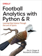
Figure 3-5. Average yards per carry plotted with seaborn

In R, create a new variable, yards per carry (ypc) and then plot the results in Figure 3-6:

## R
pbp_r_run_ave <-
    pbp_r_run |>
    group_by(ydstogo) |>
    summarize(ypc = mean(rushing_yards))

ggplot(pbp_r_run_ave, aes(x = ydstogo, y = ypc)) +
    geom_point() +
    theme_bw() +
    stat_smooth(method = "lm")

Figure 3-6. Average yards per carry plotted with ggplot2

Simple Linear Regression

Now that you’ve wrangled and interrogated the data, you’re ready to run a simple linear regression. Python and R use the same formula notation for the functions we show you in this book. For example, to build a simple linear regression where ydstogo predicts rushing_yards, you use the formula rushing_yards ~ 1 + ydstogo.

You can read this formula as rushing_yards are predicted by (indicated by the tilde, ~, which is located next to the 1 key on US keyboards and whose location varies on other keyboards) an intercept (1) and a slope parameter for yards to go (ydstogo). The 1 is an optional value to explicitly tell you where the model contains an intercept. Our code and most people’s code we read do not usually include an intercept in the formula, but we include it here to help you explicitly think about this term in the model.

We are using the statsmodels package because it is better for statistical inference compared to the more popular Python package scikit-learn that is better for machine learning. Additionally, statsmodels uses similar syntax as R, which allows you to more readily compare the two languages.

In Python, use the statsmodels package’s formula.api imported as smf, to run an ordinary least-squares regression, ols(). To build the model, you will need to tell Python how to fit the regression. For this, model that the number of rushing yards for a play (rushing_yards) is predicted by an intercept (1) and the number of yards to go for the play (ydstogo), which is written as a formula: rushing_yards ~ 1 + ydstogo.

Using Python, build the model, fit the model, and then look at the model’s summary:

## Python
import statsmodels.formula.api as smf

yard_to_go_py =
    smf.ols(formula='rushing_yards ~ 1 + ydstogo', data=pbp_py_run)

print(yard_to_go_py.fit().summary())

Resulting in:

                            OLS Regression Results
==============================================================================
Dep. Variable:          rushing_yards   R-squared:                       0.007
Model:                            OLS   Adj. R-squared:                  0.007
Method:                 Least Squares   F-statistic:                     623.7
Date:                Sun, 04 Jun 2023   Prob (F-statistic):          3.34e-137
Time:                        09:35:30   Log-Likelihood:            -3.0107e+05
No. Observations:               92425   AIC:                         6.021e+05
Df Residuals:                   92423   BIC:                         6.022e+05
Df Model:                           1
Covariance Type:            nonrobust
==============================================================================
                 coef    std err          t      P>|t|      [0.025      0.975]
------------------------------------------------------------------------------
Intercept      3.2188      0.047     68.142      0.000       3.126       3.311
ydstogo        0.1329      0.005     24.974      0.000       0.122       0.143
==============================================================================
Omnibus:                    81985.726   Durbin-Watson:                   1.994
Prob(Omnibus):                  0.000   Jarque-Bera (JB):          4086040.920
Skew:                           4.126   Prob(JB):                         0.00
Kurtosis:                      34.511   Cond. No.                         20.5
==============================================================================

Notes:
[1] Standard Errors assume that the covariance matrix of the errors is
    correctly specified.

This summary output includes a description of the model. Many of the summary items should be straightforward, such as the dependent variable (Dep. Variable), Date, and Time. The number of observations (No. Observations) relates to the degrees of freedom. The degrees of freedom indicate the number of “extra” observations that exist compared to the number of parameters fit.

With this model, two parameters were fit: a slope for rushing_yards and an intercept, Intercept. Hence, the Df Residuals equals the No. Observations–2. The $R^2$ value corresponds to how well the model fits the data. If $R^2=1.0$, the model fits the data perfectly. Conversely, if $R^2$ = 0, the model does not predict the data at all. In this case, the low $R^2$ of 0.007 shows that the simple model does not predict the data well.

Other outputs of interest include the coefficient estimates for the Intercept and ydstogo. The Intercept is the number of rushing yards expected to be gained if there are 0 yards to go for a first down or a touchdown (which never actually occurs in real life). The slope for ydstogo corresponds to the expected number of additional rushing yards expected to be gained for each additional yard to go. For example, a rushing play with 2 yards to go would be expected to produce 3.2(intercept) + 0.1(slope) × 2(number of yards to go) = 3.4 yards on average.

With the coefficients, a point estimate exists (coef) as well as the standard error (std err). The standard error (SE) captures the uncertainty around the estimate for the coefficient, something Appendix B describes in greater detail. The t-value comes from a statistical distribution (specifically, the t-distribution) and is used to generate the SE and confidence interval (CI). The p-value provides the probability of obtaining the observed t-value, assuming the null hypothesis of the coefficient being 0 is true.

The p-value ties into null hypothesis significance testing (NHST), something that most introductory statistics courses cover, but is increasingly falling out of use by practicing statisticians. Lastly, the summary includes the 95% CI for the coefficients. The lower CI is the [0.025 column, and the upper CI is the 0.975] column (97.5 – 2.5 = 95%). The 95% CI should contain the true estimate for the coefficient 95% of the time, assuming the observation process is repeated many times. However, you never know which 5% of the time you are wrong.

You can fit a similar, linear model (lm()) by using R and then print the summary results:

## R
yard_to_go_r <-
    lm(rushing_yards ~ 1 + ydstogo, data = pbp_r_run)

summary(yard_to_go_r)

Resulting in:

Call:
lm(formula = rushing_yards ~ 1 + ydstogo, data = pbp_r_run)

Residuals:
    Min      1Q  Median      3Q     Max
-33.079  -3.352  -1.415   1.453  94.453

Coefficients:
            Estimate Std. Error t value Pr(>|t|)
(Intercept)  3.21876    0.04724   68.14   <2e-16 ***
ydstogo      0.13287    0.00532   24.97   <2e-16 ***
---
Signif. codes:  0 '***' 0.001 '**' 0.01 '*' 0.05 '.' 0.1 ' ' 1

Residual standard error: 6.287 on 92423 degrees of freedom
Multiple R-squared:  0.006703,  Adjusted R-squared:  0.006692
F-statistic: 623.7 on 1 and 92423 DF,  p-value: < 2.2e-16

The general structure of the regression output differs in R compared to Python. However, the items provided are similar, with the main difference occurring in formatting. R provides the model formula, or Call, followed by a summary of the residuals. Residuals indicate how well data compares to the model’s fit. For RYOE, you actually will use the residuals later. Then the summary provides the Coefficients and their uncertainty. Last, model details are printed, which are similar to the Python details.

Lastly, before moving on to look at RYOE, we need to save the residuals to create an RYOE column in the data. Residuals are the difference between a model’s expected (or predicted) output and the observed data. With pandas in Python, create a new RYOE column in the pbp_py_run dataframe from the model’s residuals:

## Python
pbp_py_run["ryoe"] =
    yard_to_go_py
    .fit()
    .resid

Likewise, in R mutate the pbp_r_run data to create a new column, ryoe:

## R
pbp_r_run <-
    pbp_r_run |>
    mutate(ryoe = resid(yard_to_go_r))

Who Was the Best in RYOE?

Now, look at the leaderboard for RYOE from 2016 to 2022, first in total yards over expected and average yards over expected per carry. As with the passer data in Chapter 2, you will need to group by both the rusher and rusher_id because some players have the same last name and first initial.

With pandas, group by seasons, rusher_id, and rusher. Then, aggregate ryoe with the count, sum, and mean, and aggregate rushing_yards with the mean. This gives the following columns:

• The count of RYOE is the number of carries a rusher has.

• The sum of RYOE is the total RYOE.

• The mean of RYOE is the RYOE per carry.

• The mean of rushing yards is the yards per carry.

Flatten the columns and reset the index to make the dataframe easier to work with. Next, rename the columns to give them football-specific names. Lastly, query the result to print only players with more than 50 carries:

## Python
ryoe_py =
    pbp_py_run
    .groupby(["season", "rusher_id", "rusher"])
    .agg({
        "ryoe": ["count", "sum", "mean"],
        "rushing_yards": "mean"})

ryoe_py.columns = 
    list(map("_".join, ryoe_py.columns))
ryoe_py.reset_index(inplace=True)

ryoe_py =
    ryoe_py
    .rename(columns={
        "ryoe_count": "n",
        "ryoe_sum": "ryoe_total",
        "ryoe_mean": "ryoe_per",
        "rushing_yards_mean": "yards_per_carry",
    }
).query("n > 50")

print(ryoe_py.sort_values("ryoe_total", ascending=False))

Resulting in:

      season   rusher_id     rusher    n  ryoe_total  ryoe_per  yards_per_carry
1989    2021  00-0036223   J.Taylor  332  417.501295  1.257534         5.454819
1440    2020  00-0032764    D.Henry  397  362.768406  0.913774         5.206549
1258    2019  00-0034796  L.Jackson  135  353.652105  2.619645         6.800000
1143    2019  00-0032764    D.Henry  387  323.921354  0.837006         5.131783
1474    2020  00-0033293    A.Jones  222  288.358241  1.298911         5.540541
...      ...         ...        ...  ...         ...       ...              ...
419     2017  00-0029613   D.Martin  139 -198.461432 -1.427780         2.920863
122     2016  00-0029613   D.Martin  144 -199.156646 -1.383032         2.923611
675     2018  00-0027325   L.Blount  155 -247.528360 -1.596957         2.696774
1058    2019  00-0030496     L.Bell  245 -286.996618 -1.171415         3.220408
267     2016  00-0032241   T.Gurley  278 -319.803875 -1.150374         3.183453

[534 rows x 7 columns]

To print the entire table in Python once, run print(ryoe_py.query("n > 50").to_string()), something we did not do in order to save space. Alternatively, you can change the printing in your entire session by using the pandas set_option() function. For example, pd.set_option("display.min_rows", 10) would always print 10 rows.

With R, use the pbp_r_run data and group by season, rusher_id, and rusher. Then summarize() to get the number per group, total RYOE, average RYOE, and yards per carry. Lastly, filter to include only players with more than 50 carries:

## R
ryoe_r <-
    pbp_r_run |>
    group_by(season, rusher_id, rusher) |>
    summarize(
        n = n(),
        ryoe_total = sum(ryoe),
        ryoe_per = mean(ryoe),
        yards_per_carry = mean(rushing_yards)
    ) |>
    arrange(-ryoe_total) |>
    filter(n > 50)

print(ryoe_r)

Resulting in:

# A tibble: 534 × 7
# Groups:   season, rusher_id [534]
   season rusher_id  rusher        n ryoe_total ryoe_per yards_per_carry
    <dbl> <chr>      <chr>     <int>      <dbl>    <dbl>           <dbl>
 1   2021 00-0036223 J.Taylor    332       418.    1.26             5.45
 2   2020 00-0032764 D.Henry     397       363.    0.914            5.21
 3   2019 00-0034796 L.Jackson   135       354.    2.62             6.8
 4   2019 00-0032764 D.Henry     387       324.    0.837            5.13
 5   2020 00-0033293 A.Jones     222       288.    1.30             5.54
 6   2019 00-0031687 R.Mostert   190       282.    1.48             5.83
 7   2016 00-0033045 E.Elliott   344       279.    0.810            5.10
 8   2021 00-0034791 N.Chubb     228       276.    1.21             5.52
 9   2022 00-0034796 L.Jackson    73       276.    3.78             7.82
10   2020 00-0034791 N.Chubb     221       254.    1.15             5.48
# ℹ 524 more rows

We did not have you print out all the tables, to save space. However, using |> print(n = Inf) at the end would allow you to see the entire table in R. Alternatively, you could change all printing for an R session by running options(pillar.print_min = n).

For the filtered lists, we had you print only the lists with players who carried the ball 50 or more times to leave out outliers as well as to save page space. We don’t have to do that for total yards, since players with so few carries will not accumulate that many RYOE, anyway.

By total RYOE, 2021 Jonathan Taylor was the best running back in football since 2016, generating over 400 RYOE, follow by the aforementioned Henry, who generated 374 RYOE during his 2,000-yard 2020 season. The third player on the list, Lamar Jackson, is a quarterback, who in 2019 earned the NFL’s MVP award for both rushing for over 1,200 yards (an NFL record for a quarterback) and leading the league in touchdown passes. In April of 2022, Jackson signed the richest contract in NFL history for his efforts.

One interesting quirk of the NFL data is that only designed runs for quarterbacks (plays that are actually running plays and not broken-down passing plays, where the quarterback pulls the ball down and runs with it) are counted in this dataset. So Jackson generating this much RYOE on just a subset of his runs is incredibly impressive.

Next, sort the data by RYOE per carry. We include only code for R, but the previous Python code is readily adaptable:

## R
ryoe_r |>
    arrange(-ryoe_per)

Resulting in:

# A tibble: 534 × 7
# Groups:   season, rusher_id [534]
   season rusher_id  rusher         n ryoe_total ryoe_per yards_per_carry
    <dbl> <chr>      <chr>      <int>      <dbl>    <dbl>           <dbl>
 1   2022 00-0034796 L.Jackson     73      276.      3.78            7.82
 2   2019 00-0034796 L.Jackson    135      354.      2.62            6.8
 3   2019 00-0035228 K.Murray      56      122.      2.17            6.5
 4   2020 00-0034796 L.Jackson    121      249.      2.06            6.26
 5   2021 00-0034750 R.Penny      119      229.      1.93            6.29
 6   2022 00-0036945 J.Fields      85      160.      1.88            6
 7   2022 00-0033357 T.Hill        96      178.      1.86            5.99
 8   2021 00-0034253 D.Hilliard    56      101.      1.80            6.25
 9   2022 00-0034750 R.Penny       57       99.2     1.74            6.07
10   2019 00-0034400 J.Wilkins     51       87.8     1.72            6.02
# ℹ 524 more rows

Looking at RYOE per carry yields three Jackson years in the top four, sandwiching a year by Kyler Murray, who is also a quarterback. Murray was the first-overall pick in the 2019 NFL Draft and elevated an Arizona Cardinals offense from the worst in football in 2018 to a much more respectable standing in 2019, through a combination of running and passing. Rashaad Penny, the Seattle Seahawks’ first-round pick in 2018, finally emerged in 2021 to earn almost 2 yards over expected per carry while leading the NFL in yards per carry overall (6.3). This earned Penny a second contract with Seattle the following offseason.

A reasonable question we should ask is whether total yards or yards per carry is a better measure of a player’s ability. Fantasy football analysts and draft analysts both carry a general consensus that “volume is earned.” The idea is that a hidden signal is in the data when a player plays enough to generate a lot of carries.

Data is an incomplete representation of reality, and players do things that aren’t captured. If a coach plays a player a lot, it’s a good indication that that player is good. Furthermore, a negative relationship generally exists between volume and efficiency for that same reason. If a player is good enough to play a lot, the defense is able to key on him more easily and reduce his efficiency. This is why we often see backup running backs with high yards-per-carry values relative to the starter in front of them (for example, look at Tony Pollard and Ezekiel Elliott for the Dallas Cowboys in 2019–2022). Other factors are at play as well (such as Zeke’s draft status and contract) that don’t necessarily make volume the be-all and end-all, but it’s important to inspect.

Data Science Tools Used in This Chapter

This chapter covered the following topics:

• Fitting a simple linear regression by using OLS() in Python or by using lm() in R

• Understanding and reading the coefficients from a simple linear regression

• Plotting a simple linear regression by using regplot() from seaborn in Python or by using geom_smooth() in R

• Using correlations with the corr() function in Python and R to conduct stability analysis

Exercises

1. What happens if you repeat the correlation analysis with 100 carries as the threshold? What happens to the differences in r values?

2. Assume all of Alstott’s carries were on third down and 1 yard to go, while all of Dunn’s carries came on first down and 10 yards to go. Is that enough to explain the discrepancy in their yards-per-carry values (3.7 versus 4.0)? Use the coefficient from the simple linear model in this chapter to understand this question.

3. What happens if you repeat the analyses in this chapter with yards to go to the endzone (yardline_100) as your feature?

4. Repeat the processes within this chapter with receivers and the passing game. To do this, you have to filter by play_type == "pass" and receiver_id not being NA or NULL.