
4 Change workbook appearance
In this chapter
Practice files
For this chapter, use the practice files from the Excel2019SBSCh04 folder. For practice file download instructions, see the introduction.
Efficiently entering data into a workbook saves you time, but you must also ensure that your data is easy to read. Microsoft Excel 2019 gives you a wide variety of ways to make your data easier to understand. For example, you can change the font, character size, or color used to present a cell’s contents. Changing how data appears on a worksheet helps set the contents of a cell apart from the contents of surrounding cells. To save time, you can define a number of custom formats and then apply them quickly to the cells you want to emphasize.
You might also want to specially format a cell’s contents to reflect the value in that cell. For example, you could create a worksheet that displays the percentage of improperly delivered packages from each regional distribution center. If that percentage exceeds a threshold, Excel could display a red traffic light icon, indicating that the center’s performance requires attention.
This chapter guides you through procedures related to changing the appearance of data, applying existing formats to data, making numbers easier to read, changing data’s appearance based on its value, and adding images to worksheets.
Format cells
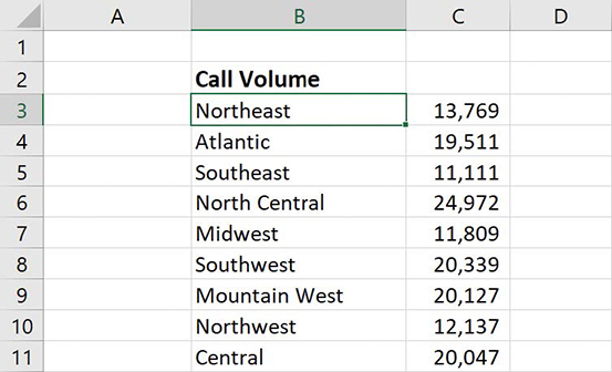
Excel worksheets can hold and process lots of data, but when you manage numerous worksheets, it can be hard to remember from a worksheet’s title exactly what data is kept in that worksheet. Data labels give you and your colleagues information about data in a worksheet, but it’s important to format the labels so that they stand out visually. To make your data labels or any other data stand out, you can change the format of the cells that hold your data.
![]() Tip
Tip
Deleting a cell’s contents doesn’t delete the cell’s formatting. To delete a selected cell’s formatting, on the Home tab, in the Editing group, click the Clear button (which looks like an eraser), and then click Clear Formats. Clicking Clear All from the same list will remove the cell’s contents and formatting.
Many of the formatting-related buttons on the ribbon have arrows at their right edges. Clicking the arrow displays a list of options for that button, such as the fonts available on your system or the colors you can assign to a cell.
![]() Tip
Tip
Clicking the body of the Border, Fill Color, or Font Color button applies the most recently applied formatting to the currently selected cells.
You can also make a cell stand apart from its neighbors by adding a border around the cell or changing the color or shading of the cell’s interior.
![]() Tip
Tip
You can display the most commonly used formatting controls by right-clicking a selected range. When you do, a mini toolbar containing a subset of the Home tab formatting tools appears above the shortcut menu.
If you want to change the attributes of every cell in a row or column, you can click the header of the row or column you want to modify and then select the format you want.
One task you can’t perform by using the tools on the ribbon is to change the default font for a workbook, used in the formula bar. The default font when you install Excel is Calibri, a simple font that is easy to read on a computer screen and on the printed page. If you’d prefer to change the default font, you can do so, but only from the Excel Options dialog box, not from the ribbon.
![]() Important
Important
The new standard font doesn’t take effect until you exit Excel and restart the app.
To change the font used to display cell contents
Select the cell or cells you want to format.
On the Home tab of the ribbon, in the Font group, click the Font arrow.
In the font list, click the font you want to apply.
To change the size of characters in a cell or cells
Select the cell or cells you want to format.
Click the Font Size arrow.
In the list of sizes, click the size you want to apply.
To change the size of characters in a cell or cells by one increment
Select the cell or cells you want to format.
Click the Increase Font Size button.
Or
Click the Decrease Font Size button.
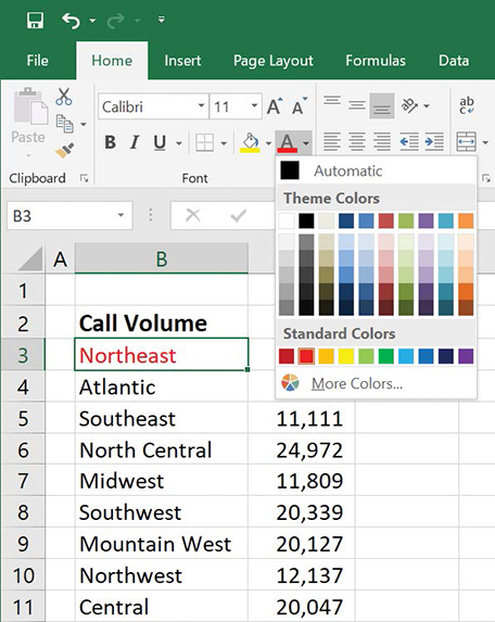
To change the color of a font
Select the cell or cells you want to format.
Click the Font Color arrow (not the button).
Click the color you want to apply.
Or
Click More Colors, select the color you want from the Colors dialog box, and then click OK.
To change the background color of a cell or cells
Select the cell or cells you want to format.
Click the Fill Color arrow (not the button).
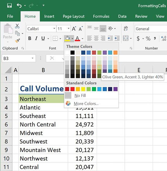
Change the fill color of a cell to make it stand out. Click the color you want to apply.
Or
Click More Colors, select the color you want from the Colors dialog box, and click OK.
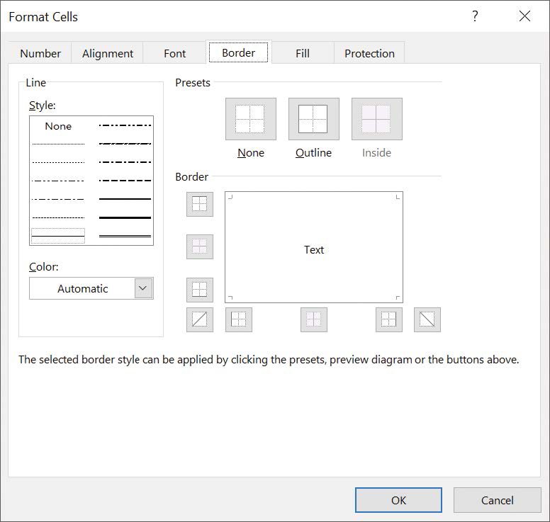
To add a border to a cell or cells
Select the cell or cells you want to format.
Click the Border arrow (not the button).
Click the border pattern you want to apply.
Or
Click More Borders, select the borders you want from the Border tab of the Format Cells dialog box, and click OK.
To change font appearance by using the controls on the Font tab of the Format Cells dialog box
Click the Font dialog box launcher.
Make the formatting changes you want, and then click OK.
To copy formatting between cells
Select the cell that contains the formatting you want to copy.
Click the Format Painter button.
Select the cells to which you want to apply the formatting.
Or
Select the cell that contains the formatting you want to copy.
Double-click the Format Painter button.
Select cells or groups of cells to which you want to apply the formatting.
Press the Esc key to turn off the Format Painter.
To delete cell formatting
Select the cell or cells from which you want to remove formatting.
In the Editing group, click the Clear button.
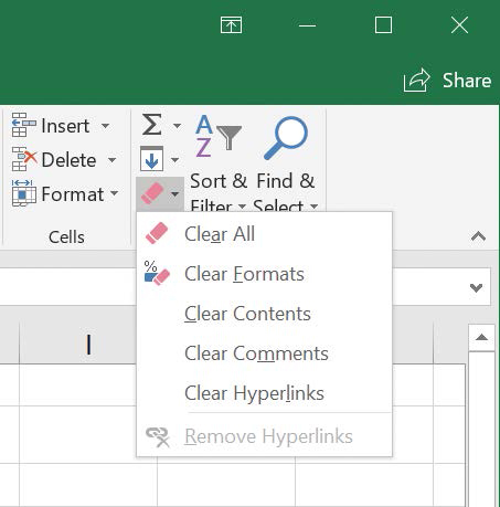
Use the Clear button to delete formats from a cell. In the menu that appears, click Clear Formats.
To change the default font of a workbook
Display the Backstage view, and then click Options.
On the General page of the Excel Options dialog box, in the Use this as the default font list, click the font you want to use.
In the Font size list, click the font size you want.
Click OK.
Exit and restart Excel to complete the default font change.
Define styles
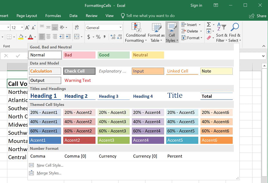
As you work with Excel, you will probably develop preferred formats for data labels, titles, and other worksheet elements. Instead of adding a format’s characteristics one element at a time to the target cells, you can format the cell in one action by using a cell style. Excel comes with many built-in styles, which you can apply by using the Cell Style gallery. You can also create your own styles by using the Style dialog box, which will appear in a separate group at the top of the gallery when you open it. If you want to preview how the contents of your cell (or cells) will look when you apply the style, point to the style to get a live preview.
![]() Tip
Tip
Depending on your screen’s resolution, cell style options might be accessed via an in-ribbon gallery instead of a Cell Styles button. If you see an in-ribbon gallery, click the More button that appears in the lower-right corner of the gallery (it looks like a small, downward-pointing black triangle) to display the full set of cell styles available.
It’s likely that any cell styles you create will be useful for more than one workbook. If you want to include cell styles from another workbook in your current workbook, you can merge the two workbooks’ style collections.
To apply a cell style to worksheet cells
Select the cells to which you want to apply the style.
On the Home tab, in the Styles group, click the Cell Styles button.
In the gallery that appears, click the style you want to apply.
To create a new cell style
Click the Cell Styles button, and then click New Cell Style.
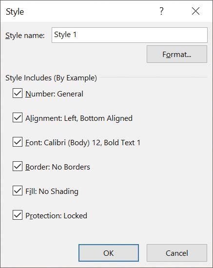
Define a custom cell style using the Style dialog box. In the Style dialog box, enter a name for the new style.
Select the check boxes next to any elements you want to include in the style definition.
Click the Format button.
Use the controls in the Format Cells dialog box to define your style.
Click OK.
To create a cell style based on existing cell formatting
Select a cell that contains the formatting on which you want to base your new cell style.
Click the Cell Styles button, and then click New Cell Style.
Excel displays the Style dialog box with the active cell’s characteristics filled in.
Enter a name for the new style.
Click OK.
To modify an existing cell style
Click the Cell Styles button, right-click the style you want to modify, and then click Modify.
In the Style dialog box, make the necessary changes to your style name and style elements.
Click the Format button.
Use the controls in the Format Cells dialog box to define your style.
Click OK.
To create a new cell style based on an existing cell style
Click the Cell Styles button, right-click the style you want to duplicate, and then click Duplicate.
In the Style dialog box, type a distinct name for the duplicate version of the style and select the elements of the existing style to include in the duplicated one.
Click the Format button.
Use the controls in the Format Cells dialog box to make any other changes to the duplicate style.
Click OK.
To merge cell styles from another open workbook
Click the Cell Styles button, and then click Merge Styles.
In the Merge Styles dialog box, click the workbook from which you want to import cell styles.
Click OK.
To delete a custom cell style
Click the Cell Styles button, right-click the style you want to delete, and then click Delete.
Apply workbook themes and Excel table styles
Excel 2019 includes powerful design tools that you can use to quickly create workbooks and worksheets that look attractive and professional. These tools include workbook themes and table styles.
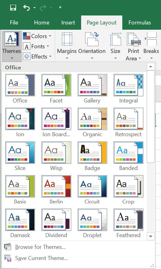
A theme is a way to specify the fonts, colors, and graphic effects that appear in a workbook. Excel comes with many themes.
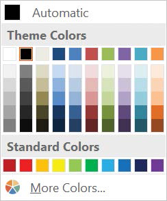
When you start to format a workbook element, Excel displays a palette of colors with two sections: standard colors, which remain constant regardless of the workbook’s theme, and colors that are available within the active theme. If you format workbook elements by using colors specific to a theme, applying a different theme changes the colors of those elements.
You can change a theme’s colors, fonts, and graphic effects. If you like the combination you create, you can save your changes as a new theme that will appear at the top of the Themes gallery.
![]() Tip
Tip
When you save a theme, you save it as an Office theme file. You can then apply the theme to other Office 2019 documents.
Just as you can define and apply themes to entire workbooks, you can apply and define Excel table styles. After you give your style a descriptive name, you can set the appearance for each Excel table element, decide whether to make your new style the default for the current document, and save your work.
![]() Tip
Tip
To remove formatting from a table element, click the name of the table element and then click the Clear button.
To apply an Office theme to a workbook
On the Page Layout tab of the ribbon, in the Themes group, click the Themes button.
Click the theme you want to apply.
To change the fonts, colors, and effects of an Office theme
In the Themes group, click the Colors, Fonts, or Effects button.
Click the set of colors, fonts, or effects you want to apply.
To create a new Office theme based on an existing theme
Use the controls in the Themes group to change the fonts, colors, or effects applied to the current theme.
Click the Themes button, and then click Save Current Theme.
Enter a name for your new theme.
Click Save.
To delete a custom Office theme
Click the Themes button, and then click Save Current Theme.
In the Save Current Theme dialog box, right-click the theme you want to delete, and then click Delete.
Click Yes.
To apply a table style
Click any cell in the list of data you want to format as a table.
On the Home tab, in the Styles group, click the Format as Table button, and then click the table style you want to apply.
In the Format as Table dialog box, verify that Excel has identified the data range correctly.
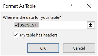
Verify that Excel has identified your table data correctly. Select or clear the My table has headers check box to reflect whether or not your list of data has headers.
Click OK.
To apply a table style and overwrite existing formatting
Click any cell in the list of data you want to format as a table.
Click the Format as Table button, and right-click the table style you want to apply.
On the shortcut menu that appears, click Apply and Clear Formatting.
Click OK.
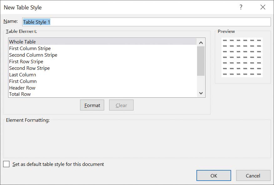
To create a new table style
Click the Format as Table button, and then click New Table Style.
In the New Table Style dialog box, enter a name for the new style.
Click the table element you want to format.
Click the Format button, change the element by using the controls in the Format Cells dialog box, and then click OK.
Repeat the previous step to change the format of other elements.
Click OK to close the New Table Style dialog box.
To modify an existing table style
Click the Format as Table button, right-click the table style you want to modify, and then click Modify.
 Important
You can’t modify the built-in Excel table styles, just the ones you create.
In the Modify Table Style dialog box, edit style elements you want to modify.
Click OK.
To delete a table style
Click the Format as Table button, right-click the table style you want to delete, and then click Delete.
ImportantYou can’t delete the built-in Excel table styles, just the ones you create.
In the message box that appears, click OK.
Make numbers easier to read
Changing the format of the cells in your worksheet can make your data much easier to read, both by setting data labels apart from the actual data and by adding borders to define the boundaries between labels and data even more clearly.
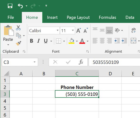
You can also make idiosyncratic data types such as dates, phone numbers, or currency values easier to read by presenting them in a standardized way, regardless of how it was entered into Excel. As an example, consider US phone numbers. These numbers are 10 digits long and have a 3-digit area code, a 3-digit exchange, and a 4-digit line number written in the form (###) ###-####. Although it’s certainly possible to enter a phone number with the expected formatting in a cell—that is, with the area code surrounded by parentheses and the exchange and digit values separated by a hyphen—it’s much more straightforward to enter a sequence of 10 digits and have Excel add those formatting elements. To do so, you indicate to Excel that the contents of the cell will be a phone number.
You can watch this format in operation if you compare the contents of the active cell and the contents of the formula box for a cell with the Phone Number formatting.
![]() Important
Important
If you enter a 9-digit number in a field that expects a phone number, you won’t get an error message. Instead, you’ll get a 2-digit area code. For example, the number 425550012 would be displayed as (42) 555-0012. An 11-digit number would be displayed with a 4-digit area code. If the phone number doesn’t look right, you probably left out a digit or included an extra one, so you should make sure your entry is correct.
Just as you can instruct Excel to expect a phone number in a cell, you can also inform Excel that a cell will contain a date or a currency amount. You can pick from a wide variety of date, currency, and other formats to best reflect your worksheet’s contents, your company standards, and how you and your colleagues expect the data to appear.
![]() Tip
Tip
You can make the most common format changes by displaying the Home tab and then, in the Number group, either clicking a button representing a built-in format or selecting a format from the Number Format list.
You can also create a custom numeric format to add a word or phrase to a number in a cell. For example, you can add the phrase per month to a cell with a formula that calculates average monthly sales for a year, to ensure that you and your colleagues will recognize the figure as a monthly average. If one of the built-in formats is close to the custom format you’d like to create, you can base your custom format on the one already included in Excel.
![]() Important
Important
You must enclose any text to be displayed as part of the format in quotation marks so that Excel recognizes the text as a string to be displayed in the cell.
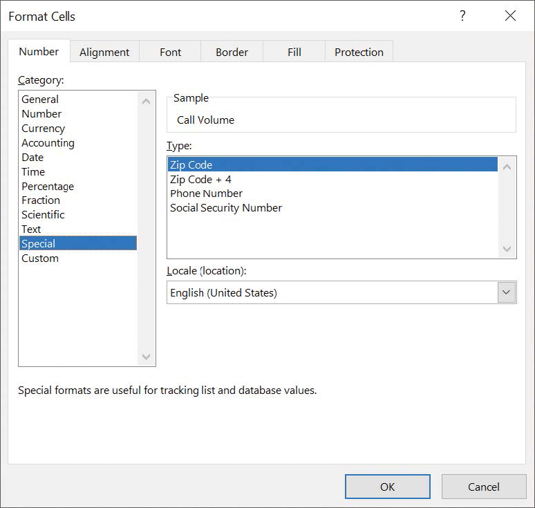
To apply a special number format
Select the cells to which you want to apply the format.
On the Home tab, in the Number group, click the Number Format arrow, and then click More Number Formats.
In the Format Cells dialog box, in the Category list, click Special.
In the Type list, click the format you want to apply.
Click OK.
To create a custom number format
On the Number Format menu, click More Number Formats.
In the Format Cells dialog box, in the Category list, click Custom.
Click the format you want to use as the base for your new format.
Edit the format in the Type box.
Click OK.
To add text to a number format
On the Number Format menu, click More Number Formats.
In the Format Cells dialog box, in the Category list, click Custom.
Click the format you want to use as the base for your new format.
In the Type box, after the format, enter the text you want to add, in quotation marks—for example, “boxes”.
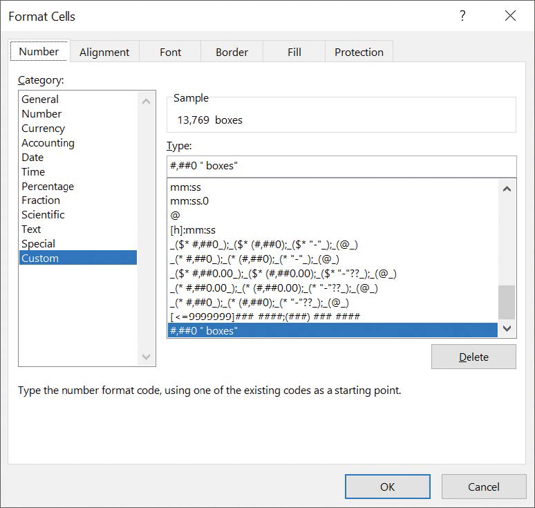
Define custom number formats that display text after values. Click OK.
Change the appearance of data based on its value
Recording information such as package volumes, vehicle miles, and other business data in a worksheet enables you to make important decisions about your operations. And as you saw earlier in this chapter, you can change the appearance of data labels and the worksheet itself to make interpreting your data easier.
Another way you can make your data easier to interpret is to have Excel change the appearance of your data based on its value. The formats that make this possible are called conditional formats, because the data must meet certain conditions, defined in conditional formatting rules, to have a format applied to it. In Excel, you can define conditional formats that change how the app displays data in cells that contain values above or below the average values of the related cells, that contain values near the top or bottom of the value range, or that contain values duplicated elsewhere in the selected range.
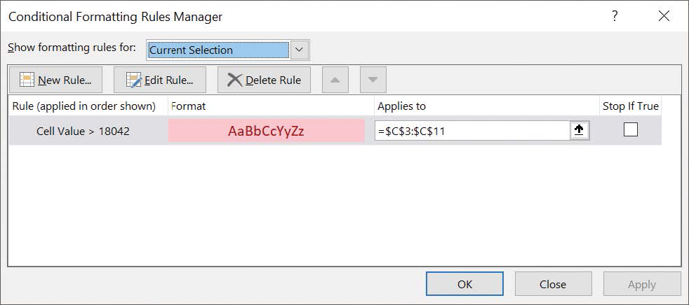
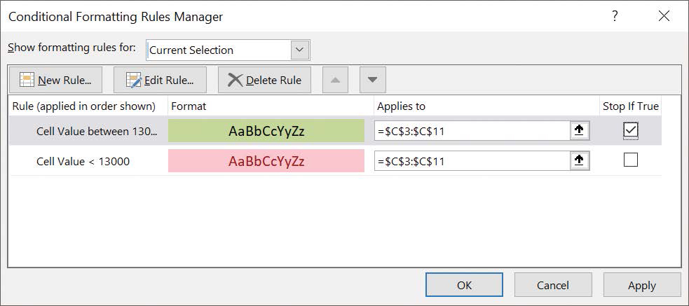
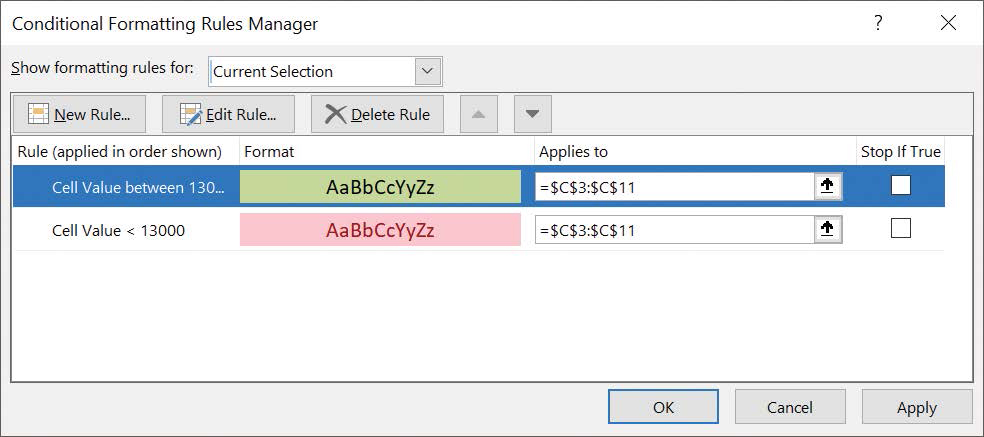
When you select which kind of condition to create, Excel displays the Conditional Formatting Rules Manager, which contains fields and controls you can use to define your rule. If your cells already have conditional formats applied to them, you can display those formats, determine the order in which they are applied, and indicate how Excel should react if more than one rule is true.
You can control your conditional formats in the following ways:
Create a new rule.
Change a rule.
Remove a rule.
Move a rule up or down in the order.
Control whether Excel continues evaluating conditional formats after it finds a rule to apply.
Save any rule changes and stop editing rules.
Save any rule changes and continue editing.
Discard any unsaved changes.
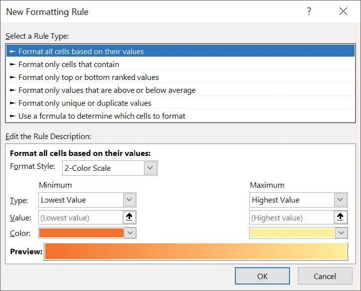
Clicking the New Rule button in the Conditional Formatting Rules Manager opens the New Formatting Rule dialog box. The commands in the New Formatting Rule dialog box duplicate the options displayed when you click the Conditional Formatting button in the Styles group on the Home tab. You can use those controls to define your new rule and the format to be displayed if the rule is true.
![]() Important
Important
Excel doesn’t check to make sure that your conditions are logically consistent, so you need to be sure that you plan and enter your conditions correctly.
You can also create three other types of conditional formats in Excel: data bars, color scales, and icon sets.
Data bars summarize the relative magnitude of values in a cell range by extending a band of color across the cell.
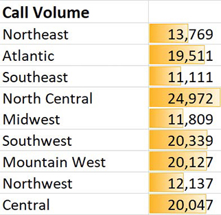
When data bars were introduced in Excel 2007, they filled cells with a color band that decreased in intensity as it moved across the cell. This pattern, called a gradient fill, made it a bit difficult to determine the relative length of two data bars because the end points weren’t as distinct as they would have been if the bars were a solid color. In Excel 2019 you can choose between a solid fill pattern, which makes the right edge of the bars easier to discern, and a gradient fill pattern, which you can use if you share your workbook with colleagues who use Excel 2007.
Excel 2019 also draws data bars differently than in Excel 2007. Excel 2007 drew a very short data bar for the lowest value in a range and a very long data bar for the highest value. The problem was that similar values could be represented by data bars of very different lengths if there wasn’t much variance among the values in the conditionally formatted range. In Excel 2019, data bars compare values based on their distance from zero, so similar values are summarized by using data bars of similar lengths.
![]() Tip
Tip
Excel 2019 data bars summarize negative values by using bars that extend to the left of a baseline that the app draws in a cell.
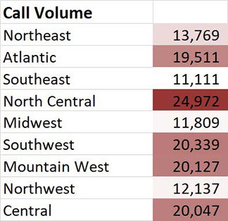
Color scales compare the relative magnitude of values in a cell range by applying colors from a two-color or three-color set to your cells. The intensity of a cell’s color reflects the value’s tendency toward the top or bottom of the values in the range.
Finally, icon sets are collections of three, four, or five images that Excel displays when certain rules are met.
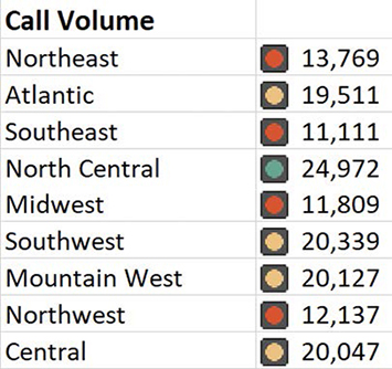
When icon sets were introduced in Excel 2007, you could apply an icon set as a whole, but you couldn’t create custom icon sets or choose to have Excel 2007 display no icon if the value in a cell met a criterion. In Excel 2019, you can display any icon from any set for any criterion or display no icon. Plus, you can edit the icon set in other ways so it summarizes your data exactly as you want it to.
When you click a color scale or icon set in the Conditional Formatting Rules Manager and then click the Edit Rule button, you can control when Excel applies a color or icon to your data.
![]() Important
Important
Do not include cells that contain summary formulas in your conditionally formatted ranges. The values, which could be much higher or lower than your regular cell data, could throw off your comparisons.
To create a conditional formatting rule
Select the cells to which you want to apply a conditional formatting rule.
On the Home tab, in the Styles group, click the Conditional Formatting button, point to Highlight Cells Rules, and then click the type of rule you want to create.
In the Conditional Formatting Rules Manager that appears, set the rules for the condition.
Click the arrow next to the with box, and then click Custom Format.
Use the controls in the Format Cells dialog box to define the custom format.
Click OK to close the Format Cells dialog box.
Click OK to close the Conditional Formatting Rules Manager.
To edit a conditional formatting rule
Select the cells to which the conditional formatting rule is applied.
Click the Conditional Formatting button, and then click Manage Rules.
In the Conditional Formatting Rules Manager, click the rule you want to edit.
Click Edit Rule.
Use the controls in the Edit Formatting Rule dialog box to change the rule settings.
Click OK twice to close the Edit Formatting Rule dialog box and the Conditional Formatting Rules Manager.
To change the order of conditional formatting rules
Select the cells to which the conditional formatting rules are applied.
Click the Conditional Formatting button, and then click Manage Rules.
In the Conditional Formatting Rules Manager, click the rule you want to move.
Click the Move Up button to move the rule up in the order.
Or
Click the Move Down button to move the rule down in the order.
Click OK.
To stop applying conditional formatting rules when a condition is met
Select the cells to which the conditional formatting rules are applied.
Click the Conditional Formatting button, and then click Manage Rules.
In the Conditional Formatting Rules Manager, select the Stop If True check box next to the rule where you want Excel to stop.
Stop checking conditional formats if a specific condition is met. Click OK.
To create a data bar conditional format
Select the range to which you want to apply the conditional format.
Click the Conditional Formatting button, point to Data Bars, and then click the format you want to apply.
To create a color scale conditional format
Select the range to which you want to apply the conditional format.
Click the Conditional Formatting button, point to Color Scales, and then click the color scale you want to apply.
To create an icon set conditional format
Select the range to which you want to apply the conditional format.
Click the Conditional Formatting button, point to Icon Sets, and then click the icon set you want to apply.
To delete a conditional format
Select the cells to which the conditional formatting rule is applied.
Click the Conditional Formatting button, and then click Manage Rules.
In the Conditional Formatting Rules Manager, click the rule you want to delete.
Delete a conditional format you no longer need. Click Delete Rule.
Click OK.
To delete all conditional formats from a worksheet
Click the Conditional Formatting button, point to Clear Rules, and then click Clear Rules from Entire Sheet.
Add images to worksheets
Establishing a strong corporate identity helps you ensure that your customers remember your organization and the products and services you offer. Setting aside the obvious need for sound management, one important attribute of a strong business is an eye-catching, easy-to-remember logo. After you or your graphic artist creates a logo, you should add an image file containing the logo to all your documents, especially any that might be seen by your customers. Not only does the logo mark the documents as coming from your company, it also serves as an advertisement, encouraging anyone who sees your worksheets to call or visit your company.
One way to add a logo or any other type of image to a worksheet is to locate the picture you want to add from your hard disk, insert it, and then make any formatting changes you want. For example, you can rotate, reposition, and resize the picture.
With Excel 2019, you can remove the background of an image you insert into a workbook. When you indicate that you want to remove an image’s background, Excel guesses which aspects of the image are in the foreground and eliminates the rest.
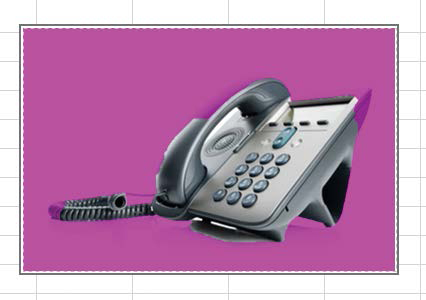
You can drag the handles on the inner square of the background removal tool to change how the tool analyzes the image.
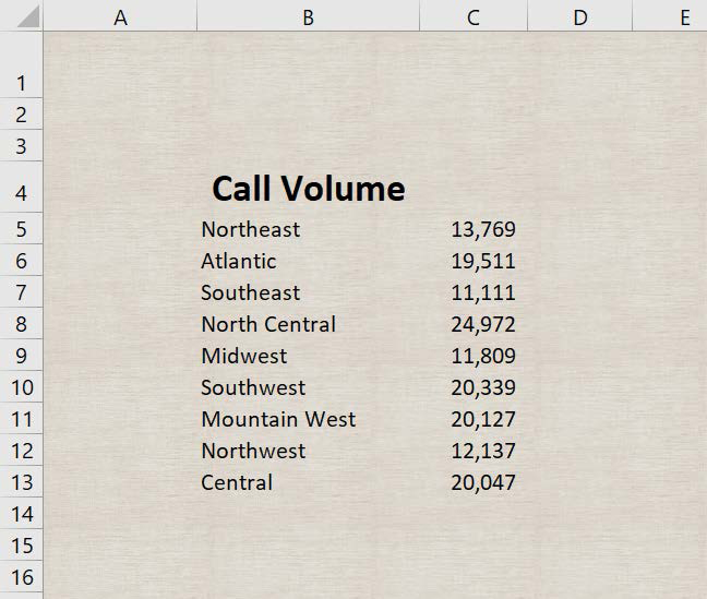
If you want to generate a repeating image in the background of a worksheet to form a tiled pattern or texture behind your worksheet’s data, or perhaps add a single image that serves as a watermark, you can do so.
![]() Tip
Tip
To remove a background image from a worksheet, display the Page Layout tab, and then in the Page Setup group, click Delete Background.
To add an image stored on your computer to a worksheet
On the Insert tab of the ribbon, in the Illustrations group, click Pictures.
In the Insert Picture dialog box, navigate to the folder that contains the image you want to add to your worksheet.
Click the image.
Click Insert.
To add an online image by using Bing Image Search
In the Illustrations group, click the Online Pictures button.
In the Insert Pictures dialog box, enter search terms identifying the type of image you want to find online.
Press Enter.
Click the image you want to add to your worksheet.
Click Insert.
To resize an image
Click the image.

Drag a handle to resize an image. Drag one of the handles that appears on the image’s border.
Or
On the Format tool tab of the ribbon, in the Size group, enter new values for the image’s vertical and horizontal size in the Height and Width boxes.
To edit an image
Click the image.
Use the controls in the Size group to change your image’s appearance.
To delete an image
Click the image.
Press the Delete key.
To remove the background from an image
Click the image.
Click the Remove Background button.
Drag the handles on the frame until the foreground of the image is defined correctly.
On the Background Removal tool tab of the ribbon, click the Keep Changes button.
To set an image as a repeating background
On the Page Layout tab, in the Page Setup group, click the Background button.
Click the Browse button and navigate to the folder that contains the file you want to use as your repeating background.
Or
Enter search terms in the Search Bing box, and then press Enter.
Click the image you want to set as your background.
Click Insert.
Skills review
In this chapter, you learned how to:
Format cells
Define styles
Apply workbook themes and Excel table styles
Make numbers easier to read
Change the appearance of data based on its value
Add images to worksheets
Practice tasks

The practice files for these tasks are located in the Excel2019SBSCh04 folder. You can save the results of the tasks in the same folder.
Format cells
Open the FormatCells workbook in Excel, and then perform the following tasks:
Change the formatting of cell B4 so the text it contains appears in 14-point, bold type.
Center the text within cell B4.
Change the background fill color of cell B4.
Draw a border around the cell range B4:C13.
Define styles
Open the DefineStyles workbook in Excel, and then perform the following tasks:
Apply an existing cell style to the values in cells B4 and C3.
Create a new cell style and apply it to the values in cell ranges B5:B13 and C4:N4.
Edit the font size of the new cell style you just created and save it under a new name.
Apply workbook themes and Excel table styles
Open the ApplyStyles workbook in Excel, and then perform the following tasks:
Display the MilesLastWeek worksheet and change the theme applied to the workbook.
Change the colors used for the new theme.
Save a new theme based on the settings currently applied to the workbook.
On the Summary worksheet, create an Excel table from the list of data in the cell range A1:B10.
Define a new Excel table style and apply it to the same data.
Make numbers easier to read
Open the FormatNumbers workbook in Excel, and then perform the following tasks:
Apply a phone number format to the value in cell G3.
Apply a currency or accounting format to the value in cell H3.
For cell H3, create a custom number format that displays the value in that cell as $255,000 plus benefits.
Change the appearance of data based on its value
Open the CreateConditionalFormats workbook in Excel, and then perform the following tasks:
Apply a conditional format to cell C15 that displays the cell’s contents with a red background if the value the cell contains is less than 90 percent.
Apply a data bar conditional format to cells C4:C12.
Apply a color scale conditional format to cells F4:F12.
Apply an icon set conditional format to cells I4:I12.
Delete the conditional format from the cell range C4:C12.
Edit the data bar conditional format so the bars are a different color.
Add images to worksheets
Open the AddImages workbook in Excel, and then perform the following tasks:
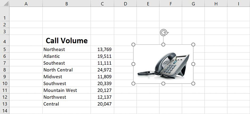
Insert the phone image file from the Excel2019SBSCh04 folder.
Remove the background from the phone image.
Resize the phone image so it will fit between the Call Volume label in cell B4 and the top of the worksheet.
Move the image to the upper-left corner of the worksheet, resizing it if necessary so it doesn’t block any of the worksheet text.
Add a repeating background image by using the texture image from the Excel2019SBSCh04 folder.