
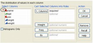
Launch Windows
The launch window is your point of entry into a platform. Table 9.1 describes three panels that all launch windows have in common.
|
Select Columns
|
Lists all of the variables in your current data table. Note the following:
• Right-click on a column name to change the modeling type.
• Filter the columns using the options in the red triangle menu. See “Columns Filter Menu”.
|
|
Cast Selected Columns into Roles
|
Moves selected columns into roles (such as Y, X, and so on.) You cast a column into the role of a variable (like an actor is cast into a role). See “Cast Selected Columns into Roles Buttons”.
This panel does not exist in the Graph Builder platform.
|
|
Action
|
OK
performs the analysis.
|
|
Cancel
stops the analysis and quits the launch window.
|
|
|
Remove
deletes any selected variables from a role.
|
|
|
Recall
populates the launch window with the last analysis that you performed.
|
|
|
Help
takes you to the Help for the launch window.
|
Cast Selected Columns into Roles Buttons
Table 9.2 describes buttons that appear frequently throughout launch windows. Buttons that are specific to certain platforms are described in the chapter for the specific platform.
|
Y
|
Identifies a column as a response or dependent variable whose distribution is to be studied.
|
|
X
|
Identifies a column as an independent, classification, or explanatory variable that predicts the distribution of the Y variable.
|
|
Weight
|
Identifies the data table column whose variables assign weight (such as importance or influence) to the data.
|
|
Freq
|
Identifies the data table column whose values assign a frequency to each row. This option is useful when a frequency is assigned to each row in summarized data. If the value is 0 or a positive integer, then the value represents the frequencies or counts of observations for each row when there are multiple units recorded.
|
|
By
|
Identifies a column that creates a report consisting of separate analyses for each level of the variable.
|
Columns Filter Menu
A Column Filter menu appears in most of the launch windows. The Column Filter menu is a red triangle within the Select Columns panel. Use these options to sort columns, show or hide columns, or search columns.
Figure 9.2 The Columns Filter Menu
|
Reset
|
Resets the columns to its original list.
|
|
Sort by Name
|
Sorts the columns in alphabetical order by name.
|
|
Continuous
|
Shows or hides columns whose modeling type is continuous.
|
|
Ordinal
|
Shows or hides columns whose modeling type is ordinal.
|
|
Nominal
|
Shows or hides columns whose modeling type is nominal.
|
|
Numeric
|
Shows or hides columns whose data type is numeric.
|
|
Character
|
Shows or hides columns whose data type is character.
|
|
Match case
|
(Only applicable to the Name options below) Makes your search case-sensitive.
|
|
Name Contains
|
Searches for column names containing specified text. To remove the text box, select Reset.
|
|
Name Does Not Contain
|
Searches for column names that do not contain specified text. To remove the text box, select Reset.
|
|
Name Starts With
|
Searches for column names that begin with specified text. To remove the text box, select Reset.
|
|
Name Ends With
|
Searches for column names that end with specified text. To remove the text box, select Reset.
|
|
Exclude Formats
|
Excludes columns with specific formats from the column selection list. Select from the following formats: date, time, geographic, or all numeric formats.
|
|
Column Groups
|
Shows or hides groups of columns. See “Group Columns” in the “Enter and Edit Data” chapter.
|
|
Ungrouped Columns
|
Shows or hides columns that have not been grouped.
|
Virtual Columns
Each launch window in JMP allows you to create one or more temporary virtual columns for use in performing analyses. These virtual columns are not part of the source data table and can only be used within the context of the current launch window. Virtual columns use formulas or calculations to define the column values. Closing the launch window or the generated report deletes any virtual columns.
Each column listed in the Select Columns pane of the launch window includes an icon representing the column’s modeling type (continuous, ordinal, or nominal) and the column name. Right-click on a column name to create a virtual column using either Transform, Combine, Aggregate, Date, Row, or Formula to calculate the column’s values.
Right-click options depend on the selected column’s data type and number of columns selected.
Figure 9.3 Example of Virtual Column Menu
Transform
For continuous and ordinal data, creates a virtual column based on a selected transcendental calculation. See “Transform Menu”.
Combine
For selected multiple continuous data, creates a virtual column based on the selected columns and calculation. See “Combine Menu”.
Aggregate
For continuous and ordinal data, creates a virtual column based on the selected aggregate function. See “Aggregate Menu”.
Date
For nominal data, creates a virtual column based on the selected date/time function. See “Date Time Menu”.
Row
For continuous, nominal, and ordinal data, creates a virtual column based on the selected row function. See “Row Menu”.
Formula
For continuous, nominal, and ordinal data, creates a virtual column containing the custom transform data based on the specified formula. See “Formula Menu”.
Note: The virtual column is only available in the current launch window. To make the virtual column available outside of the current launch window, right-click on the virtual column and select Add to Data Table. The virtual column is appended to the source data table.
Transform Menu
Select a function from the Transform menu to create a virtual column containing the calculations based on the selected function. For details on listed functions, see “Transcendental Functions” in the “Formula Functions Reference” appendix and “Numeric Functions” in the “Formula Functions Reference” appendix. Also refer to Fitting Linear Models for additional information.
Note: You can apply unary functions to multiple columns resulting in multiple virtual columns.
In addition to the functions described in the appendix, the following functions are included in the menu:
Square
Calculates the square for the selected column values.
Pow10
Calculates 10 raised to the power of the selected column values.
Cube
Calculates the cube for the selected column values.
Reciprocal
Calculates the reciprocal (1/column) for the selected column values.
Negation
Calculates the negative for the selected column values.
Combine Menu
Select multiple columns to access the Combine menu. The Combine menu creates a virtual column containing the calculations based on the selected function. For details on listed functions, see “Statistical Functions” in the “Formula Functions Reference” appendix.
In addition to the functions described in the appendix, the following functions are included in the menu:
Difference
Calculates the difference between the first and second columns (A - B).
Difference (reverse order)
Calculates the difference between the second and first columns (B - A).
Ratio
Calculated the ratio of the first column to the second column (A / B).
Ratio (reverse order)
Calculates the ratio of the second column to the first column (B / A).
Average
Returns the average value of the selected columns.
Aggregate Menu
Select a function from the Aggregate menu to create a virtual column containing the statistics calculated from the selected column (or part of a column if you specified a Group By column). For details on listed functions, see “Statistical Functions” in the “Formula Functions Reference” appendix.
Note: The Group By option is useful for these functions.
In addition to the functions described in the appendix, the following functions are included in the menu:
Count
Calculates the number of values in the selected column.
Median
Calculates the median value for the selected column
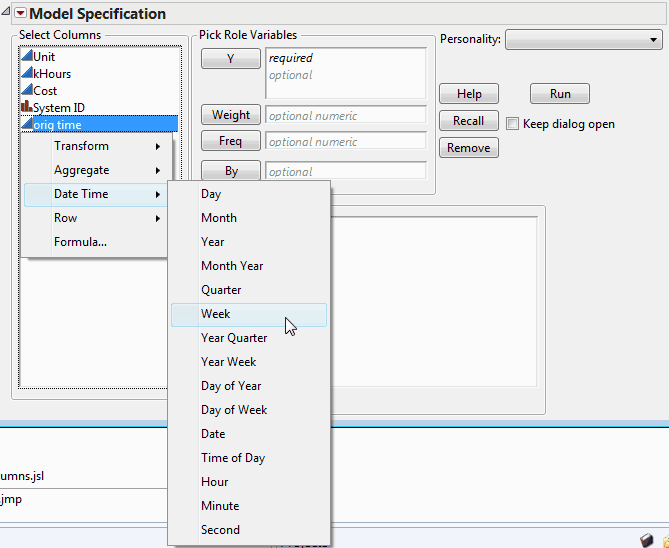
Date Time Menu
For column values containing date or time values, select a function from the Date menu to create a virtual column containing values calculated from the selected column. For details on listed functions, see “Date Time Functions” in the “Formula Functions Reference” appendix.
In addition to the functions described in the appendix, the following functions are included in the menu:
Month Year
Returns the month number and year for the date in the selected column.
Week
Returns the number of the week in the year for the date in the selected column.
Year Quarter
Returns the year and the year’s quarter (1, 2, 3, or 4) for the date in the selected column.
Year Week
Returns a string representing the ISO-8601 week of year format (for example, June 12, 2013 results in “2013W24”).
Character Menu
Select a function from the Character menu to create a virtual column containing strings formed by the selected Character function. For details on listed functions, see “Character Functions” in the “Formula Functions Reference” appendix.
In addition to the functions described in the appendix, the following functions are included in the menu:
Concatenate with Space
Concatenates the strings in the selected column or columns into a new string with each sub-string separated by a whitespace.
Concatenate with Comma
Concatenates the strings in the selected column or columns into a new string with each sub-string separated by a comma character.
First Word
Extracts the first word from a character string in the selected column or columns.
Last Word
Extraacts the last word from a character string in the selected column or columns.
Row Menu
Select a function from the Row menu to create a virtual column containing calculations determined by the selected Row function. For details on listed functions, see “Row Functions” in the “Formula Functions Reference” appendix and “Random Functions” in the “Formula Functions Reference” appendix.
See the Scripting Guide book for details on Row functions.
In addition to the functions described in the appendix, the following functions are included in the menu:
Difference
Calculates the difference of each value in the selected column using the formula:
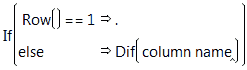
Note: The Difference function also supports the Group By option.
Cumulative Sum
Calculates the cumulative sum for each value in the selected column using the formula:
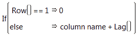
Note: The Cumulative Sum function also supports the Group By option.
Moving Average
Calculates the exponentially weighted moving average, EWMA, (given a smoothing parameter in the range of 0 to 1.0) for each value in the selected column using the formula:
Formula Menu
Select Formula to create a virtual column using a formula. See “Create a Formula” in the “Formula Editor” chapter for details on creating and editing a formula.
Note: JMP evaluates the formula entered on-demand therefore complex formulas may require a lot of processing time.
Virtual Column Options
After creating a virtual column, you can perform the following actions:
Rename
Renames the virtual column.
Add to Data Table
Adds the virtual column to the data table as a formula column.
Remove Transform Column
Removes the virtual column from the launch window.
Group By
Specifies the column to use for grouping data analysis (that is, all analyses are performed separately for each level of the specified column).
Platforms that Support Multithreading
Some platforms in JMP are coded to take advantage of multiple CPU's on a machine, allowing these platforms to run significantly faster. This process is called multithreading.
As of JMP 11, the following platforms support multithreading:
• Choice
• Distribution
• Factor Analysis
• Fit Life by X
• Fit Model: Parametric Survival, Mixed Model  , Generalized Regression
  , and Response Screening
• Life Distribution
• Multivariate
• Neural
• Nominal Logistic
• Nonlinear and Nonlinear Curve
• Partial Least Squares 
• Partition
• Principal Components
• Profiler (does not apply to Profilers launched from within other platforms)
• Reliability Forecast
Navigating Reports
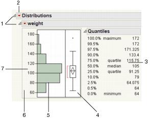
JMP reports are displayed in standard windows with scroll bars and options to resize. They also have other special buttons and menus like those illustrated in Figure 9.4 and those discussed in the following sections.
Figure 9.4 Basics of the Report Window
|
Number
|
Action
|
|
1
|
Click on the disclosure buttons to hide or show sections of the report.
|
|
2
|
Click on the red triangle menus to access report options.
|
|
3
|
Right-click in the table to access formatting options.
|
|
4
|
Click and drag on the borders to resize graphs.
|
|
5
|
Right-click anywhere in the graph to access formatting options.
|
|
6
|
Right-click within the axis to access formatting options.
|
|
7
|
The arrow cursor turns into a hand when you hover over an axis. Click and drag using to scroll along the axis or to rescale the axis. See “Scroll and Scale Axes”.
|
Use the Hand Tool
Select the hand tool using the Tools > Grabber option. There are many functions that you can use with the hand tool (also known as the grabber tool) in a report. Here are some examples of the way the hand behaves in graphs and plots:
• On histograms, for continuous variables, use the hand tool to change the number of bars or to shift the boundaries of the bars.
• In all report tables, use the hand tool to click and drag columns for rearranging.
• Use the hand tool to change the displayed range of axis values. See “Scroll and Scale Axes”.
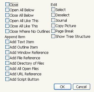
Access Report Display Options
Right-click a disclosure button  to show a menu that lets you rearrange the report and gives you control over report outline levels. The resulting menu has the following report formatting options:
Close
Closes (hides) that section of the report. This can also be accomplished by clicking the disclosure button.
Horizontal
if available, the option switches the outline of the report between a vertical and horizontal layout.
Open All Below
Opens all outline levels beneath the level where this command is selected, including that level.
Close All Below
Closes all outline levels beneath the level where this command is selected, including that level.
Open All Like This
Opens all of the same type of reports as the one that is present in the analysis window. If you analyze several variables at a time, you often want to open many of the same type of report tables all at once. You might also want to open all of the same type of report tables at once when you select multiple options on a single analysis.
Close All Like This
Closes all of the same type of reports as the one that is present in the analysis window.
Close Where No Outlines
Closes all parts of the report that do not have sublevels. This command is usually used at the top level of the report outline. It is a quick way to see a nesting structure overview of a report.
Append Item
Displays a submenu, which lists ways that you can add structural items to the report. Items include text, outline title bars, references to other JMP files and windows, a list of all open JMP files, and URLs.
Edit
Displays the submenu shown in Figure 9.5, which affect all reports at the outline level where they are used:
Select
Highlights all reports for that outline level.
Deselect
Deselects all selected reports for that outline level.
Journal
Duplicates the report in a separate window titled Journal so you can edit it or append other reports to it. See “JMP Journals” in the “Save and Share Data” chapter.
Copy Picture
Copies the report to the clipboard. You can then open another application and paste it.
Page Break
Inserts a page break for printing purposes.
Show Tree Structure
Opens a window that shows the DisplayBoxes that make up the report. This is mainly used by JSL programmers who are manipulating or reading parts of the report. See the Display Trees chapter in the Scripting Guide book for details.
An alternative way to access these options is to hold down the ALT key and right-click the disclosure button . This displays a window, as shown in Figure 9.5, with check boxes for commands and options so that you can select multiple actions at the same time. You can also do the same for the menu under a red triangle menu.
Figure 9.5 Menu Items in a Window
Show and Hide Parts of a Report
JMP reports are organized in a hierarchical outline. Each level of the outline has a triangle-shaped disclosure button . Click the disclosure button to open and close that section of the report.
Combine Several Reports
Suppose that you perform multiple analyses and want to show all of the results (and the data table) in one window. You can select and combine the reports and the data table in several ways.
Note: Most JMP windows can be combined (reports, data tables, scripts, journals, etc.) Look for the empty check box in the lower right corner of each window.
On Windows:
• Right-click the windows that you want to combine in the Home Window or Window List and then select Combine.
• Select the check box in the lower right corner of the windows that you want to combine, then select Combine selected windows next to the check box. Or, select the corresponding commands in the Window > Arrange menu.
On Mac:
1. Select Window > Combine Windows.
2. Select the windows that you want to combine and click OK.
In the combined window, using the options in the Report red triangle menu, you can:
• Edit the existing layout in the Application Builder
• Save the script to a data table, journal, script window, or as an add-in.
Rename a Title
To rename a title in a report, double-click on any of the following titles:
• a title next to a red triangle menu
• a title next to a disclosure button
• a column title
Increase Font Sizes
On Windows, change the font size that JMP uses in reports and data tables by selecting Window > Font Sizes. Then choose from one of the submenu items:
Increase Font Size
Increases the font size. Select again to increase the font size again.
Decrease Font Size
Decreases the font size. Select again to decrease the font size again.
How to Access Analysis Options
Click the red triangle menu in a report to access a list of options that apply for that particular report. In addition to clicking the red triangle menu, you can also:
• Select multiple actions at the same time. Hold down the ALT key and click the red triangle menu. A panel of all commands and options appears with check boxes.
• Apply a command to all similar reports in the report window. Hold down the CTRL key and click the red triangle menu. For example, in a One-way analysis, if you hold down the CTRL key, click the icon, and select Means/Anova/t Test, an analysis of variance is performed for all One-way analyses in the active report window.
The red triangle options applicable to each platform in the Analyze and Graph menus are described in the following books:
• Basic Analysis
• Essential Graphing
• Multivariate Methods
• Fitting Linear Models
• Specialized Models
• Quality and Process Methods
• Reliability and Survival Methods
Script Menus
The red triangle menu at the top level of every JMP report contains a Script menu. Most of these options are the same throughout JMP. A few platforms add extra options that are described in the specific platform chapters. Table 9.4 lists the Script menu options that are common to all platforms.
|
Redo Analysis
|
If the values in the data table that was used to produce the report have changed, this option duplicates the analysis based on the new data. The new analysis appears in a new report window.
|
|
Relaunch Analysis
|
Opens the platform Launch window and recalls the settings used to create the report.
|
|
Automatic Recalc
|
Automatically updates analyses and graphics when data table values change. See “Automatic Recalc”.
|
|
Copy Script
|
Places the script that reproduces the report on the clipboard so that it can be pasted elsewhere.
|
|
Save Script to Data Table
|
Saves the script to the data table that was used to produce the report.
|
|
Save Script to Journal
|
Saves a button that runs the script in a journal. The script is added to the current journal.
|
|
Save Script to Script Window
|
Opens a script editor window and adds the script to it. If you have already saved a script to a script window, additional scripts are added to the bottom of the same script window.
|
|
Save Script to Report
|
Adds the script to the top of the report window.
|
|
Save Script for All Objects
|
If you have By groups or similar multiple reports, a script for each object is saved to the script window. Otherwise, this option is the same as Save Script to Script Window.
|
|
Save Script to Project
|
Saves the script in a project. If you have a project open that contains the report, the script is added to that project. If you do not have a project that contains the report, a new project is created and the script is added to it.
|
|
Data Table Window
|
Brings the corresponding data table used to create the report to the front.
|
|
Local Data Filter
|
If your data table contains row states and you do not want to affect them, use the Local Data Filter. The actions of this data filter are temporary and you can experiment with it.
Note: Platforms that do not support the Automatic Recalc option also do not support the Local Data Filter option.
|
|
Column Switcher
|
Lets you interactively exchange one column for another on a graph. See “Column Switcher”.
|
If you have specified a By variable in the platform launch window, the Script All By-Groups menu also appears. These options apply to the reports for all the levels of the By variable.
|
Redo Analysis
|
If the values in the data table that was used to produce the reports have changed, this option duplicates the analysis based on the new data and produces new reports.
|
|
Relaunch Analysis
|
Opens the platform Launch window and recalls the settings used to create the reports.
|
|
Copy Script
|
Places the script that reproduces the reports on the clipboard so that it can be pasted elsewhere.
|
|
Save Script to Data Table
|
Saves the script to the data table that was used to produce the reports.
|
|
Save Script to Journal
|
Saves a button that runs the script in a journal. The script is added to the current journal.
|
|
Save Script to Script Window
|
Opens a script editor window and adds the script to it. If you have already saved a script to a script window, additional scripts are added to the bottom of the same script window.
|
Automatic Recalc
The Automatic Recalc feature immediately reflects changes that you make to the data table in the corresponding report window. You can make any of the following data table changes:
• exclude or unexclude data table rows
• delete or add data table rows
This powerful feature immediately reflects these changes to the corresponding analyses, statistics, and graphs that are located in a report window.
To turn on Automatic Recalc for a report window, click on the platform red triangle menu and select Script > Automatic Recalc. To turn it off, deselect the same option. You can also turn on Automatic Recalc using JSL.
Note the following:
• By default, Automatic Recalc is turned off for platforms in the Analyze menu and turned on for platforms in the Graph menu. The exceptions are the Capability, Variability/Gauge Chart, and Control Chart > Run Chart platforms.
• For some platforms, the Automatic Recalc feature is not appropriate and therefore is not supported. These platforms include the following: DOE, Profilers, Choice, Partition, Nonlinear, Neural, Neural Net, Partial Least Squares, Fit Model (REML, GLM, Log Variance), Gaussian Process, Item Analysis, Cox Proportional Hazard, and Control Charts (except Run Chart).
Column Switcher
Within a report, use the Column Switcher to quickly analyze different variables without having to recreate your analysis. To activate the Column Switcher, from a report window, click on the red triangle menu. Select Script > Column Switcher.
If you have multiple columns, use the buttons to animate the column switching or step through each column manually. Move the slider control to change the speed of the animation.
Example of the Column Switcher
You have data about nutrition information for candy bars. You want to examine different factors, to see which factors best predict calorie levels.
1. Open the Candy Bars.jmp sample data table.
2. Select Graph > Graph Builder.
3. Click Total fat g and drag to the X zone.
4. Click Calories and drag to the Y zone.
5. Click Cholesterol g and drag to the Wrap zone.
6. From the red triangle next to Graph Builder, select Script > Column Switcher.
Choose the column that you want to switch from:
7. Select Cholesterol g and click OK.
Choose the columns that you want to switch to:
8. Select Saturated fat g, Cholesterol g, Sodium mg, Carbohydrate g, Dietary fiber g, and Sugars g and click OK.
Figure 9.6 Column Switcher in Graph Builder Window
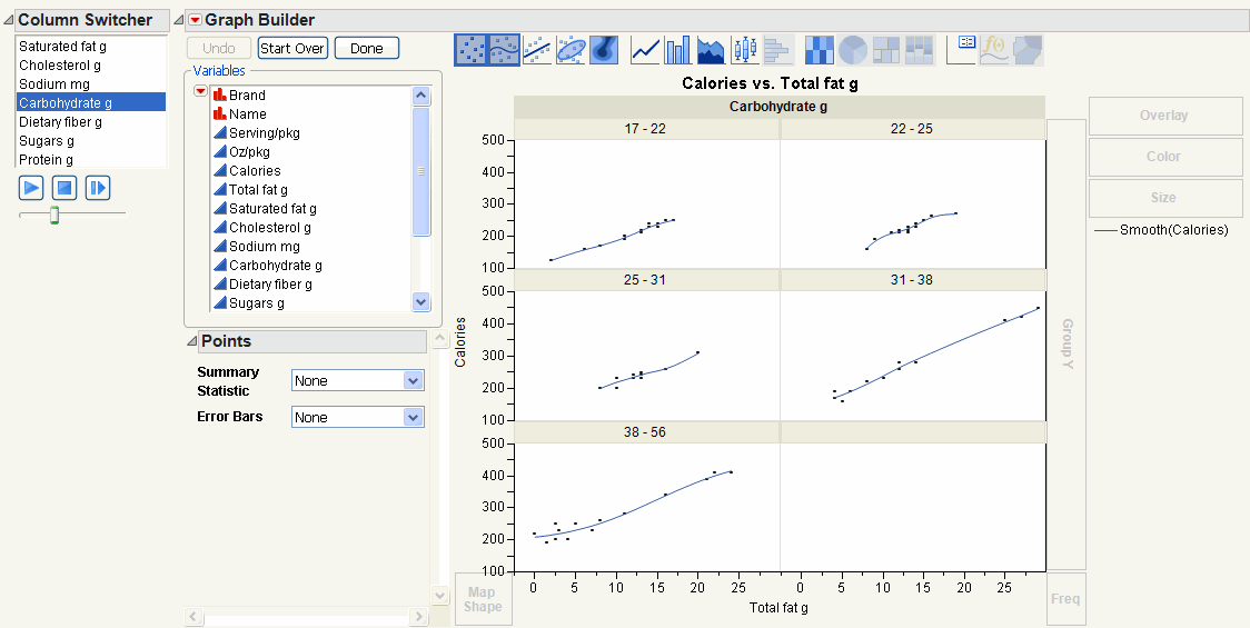
9. Click the Play button to cycle between the different factors. Use the slider to control the speed of the animation. Alternatively, you can step through each factor individually.
You can see that the relationship between calories and fat is relatively strong for each level of carbohydrate. Therefore, Carbohydrate g appears to be the best predictor of calorie levels.
..................Content has been hidden....................
You can't read the all page of ebook, please click here login for view all page.