
Chapter 4
Iris Biometric Data Indexing
Iris biometric-based identification system deals with high dimensional complex features. Hence, the searching with these features makes the identification process extremely slow as well as increases the false acceptance rate beyond an acceptable range. To improve the efficiency of an iris-based identification system, an indexing mechanism has been proposed. In this chapter, the indexing technique with low dimensional feature vector for an iris-based biometric identification system is described. The method is based on the iris texture features. Gabor energy features of iris texture are computed to create a twelve dimensional index key vector. A new storing structure and retrieving technique have been proposed to store and retrieve the iris data from the database. The block diagram of the iris biometric data indexing method is given in Fig. 4.1. The different tasks involved in this approach are discussed in this chapter.
The rest of the chapter is organized as follows. An overview of Gabor filter will be discussed in Section 4.1. In Section 4.2, the preprocessing technique for iris image is described. Section 4.3 will describe the feature extraction technique for iris biometric. A new index key generation method for iris biometric data will be introduced in Section 4.4. The storing and retrieving techniques of iris data shall be given in Section 4.5 and Section 4.6, respectively. The performance evaluation of the indexing method will be presented in Section 4.7. The comparison with existing work will be reported in Section 4.8. Finally, Section 4.9 will give the summary of this chapter.

Figure 4.1: An overview of the proposed iris biometric data indexing approach.
4.1 Preliminaries of Gabor Filter
Gabor filter is used in this work. For better understanding of work, the concept of the Gabor filter is breifly discussed in this section.
Gabor transform theory was first proposed by D. Gabor in 1946 [16]. Daugman [8] proposed two-dimensional (2-D) Gabor transform theory in 1985. It has been observed that the 2-D Gabor filter is an effective method for time-frequency analysis [8, 10]. In the spatial domain, a 2-D Gabor filter consists of a sinusoidal wave modulated by a Gaussian envelope. It performs a localized and oriented frequency analysis of a 2-D signal.
A 2-D Gabor function g(x, y) and its Fourier transform G(u, v) can be expressed as in Eq. (4.1) and Eq. (4.2) [19, 23], respectively.


where, σu = 1/2πσx and σv = 1/2πσy. In Eq. (4.1), σx and σy are the standard deviations of the Gaussian envelope along x and y directions, respectively and determine the filter bandwidth. Here, (x, y) and (u, v) are the spatial domain and frequency domain coordinates, respectively. W is the center frequency of the filter in frequency domain and j is called the imaginary unit, where ![]() .
.
A multi-resolution Gabor filter (also called multi-channel Gabor wavelet) is a set of filter banks with different scales (frequencies) and orientations. The Gabor filter forms a complete but nonorthogonal basis set. Expanding a signal using this basis provides a localized frequency description, thus capturing local features or energy of the signal. Texture features can then be extracted from this group of energy distributions. The Gabor wavelet can be represented with a mother wavelet and derived the appropriate Gabor functions by different rotations and scales. Let g(x, y) be the mother wavelet of the Gabor filter family. The set of Gabor filter bank gm,n(x, y) can be generated from g(x, y) as expressed in Eq. (4.3).
where a is a constant such that a > 1, m, n are two integer variables, and x′ and y′ are represented in Eq. (4.4).

In Eq. (4.4), θn = nπ/K, m = 0, 1, . . . , S–1, and n = 0, 1, . . . , K − 1. The parameters S and K are the total number of scales and orientations in the multi-resolution decomposition, respectively. The values of S and K are to be chosen to ensure that the half-peak magnitude support of the filter responses in the frequency spectrum touch each other. The filter parameters a, σu and σv can be computed as follows:

(4.5)
where Ul and Uh denote the lower and upper center frequencies of interest, respectively.
The Gabor feature space consists of responses calculated with a multi-resolution Gabor filter at several different scales (frequencies) and orientations. The response of a Gabor filter to an image is obtained by a 2-D convolution. Convolution of an image with the kernel gives a response that is proportional to how well the local features in the image match the kernel. Let I(x,y) denotes an image and GIm,n(x, y) denotes the response of a Gabor filter at the mth scale and nth orientation to an image point (x, y). The Gabor filter response to an image is defined in Eq. (4.6).

The Gabor filtered image has both real and imaginary components, as the response of the Gabor filter is complex. The magnitude of the Gabor filtered image is calculated by using Eq. (4.7).
where ReGIm,n(x, y) and ImGIm,n(x, y) are the real and imaginary parts of the Gabor filtered image, respectively.
In this work, multi-resolution Gabor filter is used to extract features from iris images.
4.2 Preprocessing
Iris localization and normalization are used as preprocessing tasks for a captured eye image. First, in localization, the iris part is isolated from an eye image. To localize the iris part, the eye image is preprocessed by applying downscaling and color level transform. The downscaling of the eye image is done to reduce the search area for pupil and iris boundaries. The original eye image is with the resolution 320×280 and the eye image is downscaled to the resolution 160×140. Figure 4.2(a) shows a sample eye image. The color level transform is applied to minimize the influence of irrelevant edges. In other words, the color level transform increases the intensity differences between the pupil and iris parts, and iris and sclera parts which in turn helps to detect the pupil and iris boundaries efficiently and accurately [12, 13]. The next step is to find the pupil boundary. To detect the pupil boundary, the color level transformed image is converted to a binary image and all connected components in the binary image are found. Then, the small irrelevant components which may occur due to eyelashes, eyelids and noise are removed. Pupil component is selected by counting the number of pixels within the calculated average radius. The pupil boundary is found from the pupil component by edge detection and edge connection. The pupil centroid is determined by calculating the centroid of all pixels within the pupil boundary. Figure 4.2(b) shows an eye image with detected pupil.
Iris boundary detection is the next step in the iris localization. To detect the iris boundary, the eye image is divided into left and right images at the pupil centroid. Color level transform is applied on both left and right images to enhance the contrast between iris and sclera boundaries. The image preprocessing technique, namely dilation [17], is followed to color level transformed image to reduce the noise effect in edge detection. The dilated image is then thresholded to create a binary image and to detect the vertical edges which mainly occur due to iris boundary. Irrelevant edges which occur due to noise and eyelashes are ,removed after the edge detection. Iris boundary and eyelid boundary are detected by checking the pixel connectivity and drawing the small lines in particular directions. Figure 4.2(c) shows detected iris boundary in the eye image. Finally, resizing of pupil and iris boundary information is done. The detected iris part is shown in Fig. 4.2(d). Detailed of the pupil and iris boundary detection have been reported in [12, 13].

Figure 4.2: Preprocessing result of a sample iris image [12, 14].
After completion of iris localization, the iris part is wrapped into a fixed size rectangular block to make the iris sample scale and translation invariant. This process is called iris normalization. A detailed about iris image normalization technique can be found in [14]. The wrapping process is done by transforming the iris texture from Cartesian to polar coordinate. The Daugman’s homogeneous rubber sheet model [11] is applied to normalize the iris texture. The normalized iris image is shown in Fig. 4.2(e). Then the normalized iris is enhanced to make the iris texture illumination invariant by applying Ma et al. [21] technique. This enhanced image is used in the feature extraction. An example of an enhanced normalized iris image is shown in Fig. 4.2(f).
4.3 Feature Extraction
Gabor energy features are extracted in different scales and orientations from a normalized iris image as stated in this section. It is known that the response of a Gabor filter to an image is obtained by a 2-D convolution operation. Let I(x,y) be the normalized iris image and GIm,n(x, y) denotes the response of Gabor filter in the mth scale and nth orientation to an image at point (x, y) on the image plane. The Gabor filtered image can then be obtained using Eq. (4.6) as stated in Section 4.1.
This approach uses the multi-resolution Gabor filter to extract the iris texture features. For this purpose, the Gabor filter is applied in each scale and orientation, and the responses are computed at each pixel of the image. These responses are called Gabor coefficient values which are complex. The magnitude values are calculated at each pixel of the image. The Gabor energy is estimated by summing up the square values of the magnitude of Gabor responses at each pixel as expressed in Eq. (4.8).
It is observed that the range of values of Gabor energy features is very high. It is also examined that intra-feature range distribution is higher for lower values of m and n. A non-linear function such as log is used to make the intra-feature range distribution similar. It effectively maps the high range of Gabor energy features’ values to a lower range of values. Thus, for a given iris image the Gabor energy features can be represented in the form of a matrix as shown in Eq. (4.9).

The rows and columns denote the number of scales (S) and number of orientations (K) of the multi-resolution Gabor filter. It may be noted that the feature vector in our approach consists of S × K number of features.
4.4 Index Key Generation
The extracted Gabor energy features in different scales and orientations are used to generate a key for iris database indexing. In this approach, a key represents a feature vector which consists of S × K number of features’ values. The ith value of an index key is denoted as f (i) in Eq. (4.10).
where GFm,n represents the logarithm value of the Gabor energy feature in the mth scale and nth orientation. In Eq. (4.10), m = 0, 1, . . . , S − 1 and n = 0, 1, . . . , K – 1, and i = n + (m × K ) + 1. In other words, the ith feature of an index key represents the logarithmic value of a Gabor energy feature in a particular scale and orientation. Note that the length of the index key is S × K which is denoted as FL. Suppose, there are P number of subjects and for each subject there are Q number of samples. The index key for the qth sample of the pth subject is denoted by Eq. (4.11) where fp,q(i) represents the ith feature of the qth sample of the pth subject, q = 1, 2, . . . , Q and p = 1, 2, . . . , P .
4.5 Storing
To store the iris data, first, an index space is created in the database, and then the iris data are stored into that index space of the database. The descriptions of creating index space and storing mechanism are discussed in the following sub sections.
4.5.1 Index Space Creation
For a given iris image, index keys are created as mentioned in Section 4.4. An index organization is proposed to store any index key for any sample. The index organization is shown in Fig. 4.3. The organization consists of FL number of tables. Each table is corresponding to each feature of the index key. The length of a table for a feature depends on the minimum and maximum values for all samples of all subjects. Thus, the length of the table for the ith feature is calculated using Eq. (4.12).
where ![]() and
and ![]() are the maximum and minimum values for all samples of all subjects of the ith feature, and i varies from 1 to FL. The
are the maximum and minimum values for all samples of all subjects of the ith feature, and i varies from 1 to FL. The ![]() and
and ![]() are then calculated using Eq. (4.13). The index value of the table corresponding to the ith feature is started with 1 and end with TLi.
are then calculated using Eq. (4.13). The index value of the table corresponding to the ith feature is started with 1 and end with TLi.


Figure 4.3: Index space organization.
Each entry of a table contains two lists (see Fig. 4.3). The list MDL contains a set of values which are calculated as the median values of all samples of a subject for a feature representing the table. The list IDL contains a set of identities which uniquely identify an iris sample.
4.5.2 Storing Iris Data
To store the index keys in the database, the values of a feature corresponding to all given samples of a subject are sorted. Then the center value of the feature values for that subject is calculated. Note that median or mean value can give the center value. The median value gives the central position which minimizes the average of the absolute deviations. On the other hand, the mean value gives the center position biasing toward the extreme value. For example, if any feature value is very low or very high for a particular sample, then the mean value is close to that feature value of the sample. Hence, the median value is used in this approach. For any ith feature, the median value of a given Q number of samples for a subject say p is calculated using Eq. (4.14).
Note that if there are P number of subjects and each subject has Q number of samples, then N = P × Q number of median values and the identities are stored in each table.
Let the unique identifier for the qth sample of the pth subject is denoted as ![]() and the ith feature value is denoted as fp,q(i). The median value and
and the ith feature value is denoted as fp,q(i). The median value and ![]() corresponding to the fp,q(i) are stored at the ti th position in the ith table. Given the value of fp,q (i), the value of index say ti, in the ith table is calculated using Eq. (4.15).
corresponding to the fp,q(i) are stored at the ti th position in the ith table. Given the value of fp,q (i), the value of index say ti, in the ith table is calculated using Eq. (4.15).
To enroll an additional samples of a subject which is already enrolled in the database, the median value of all enrolled samples with the additional samples for that subject is recalculated. Then, the all samples of the subject are enrolled into the database. If a new subject comes to enroll, first, the median value of each feature for all samples of the new subject is calculated. Then, the minimum and maximum values of each feature are checked to confirm whether the values are within the range of the table or not. If feature values lie within the range of the table then the identity and the median value of the new subject are enrolled. If the values do not fall within the range, then the size of table is increased with the new minimum and maximum values and the enrolled samples are reorganized. Finally, all samples of the new subject are enrolled.
Illustration: The approaches to store and index iris biometric data are illustrated with an example. Suppose, there are data of 10 subjects with 5 sample each. Thus, the total number of samples to be stored and indexed is 50. Further, 3 scales and 4 orientations are considered for Gabor feature extraction. Hence, the length of the index key is 12. That is, 12 tables are needed in the database to store the 12 features for each index key. The index keys for 50 samples are created as discussed in Section 4.4. Figure 4.4 shows the index keys of 5
samples and all data pertaining to say, sixth subject for an instance. Let assume that the minimum and maximum values of the first feature analyzing all fifty samples are found to be 100 and 350, respectively. Thus, the length of the first table in the database is 251 (Fmax1 − Fmin1 + 1). Similarly, the length of the other tables in the database can be calculated from the maximum and minimum values of features. Now, the first sample of the sixth subject needs to be enrolled into the database. Among all the index keys of the sixth subject, the first sample is highlighted as shown in Fig. 4.4. Now, the median value for each feature of the sixth subject is to be found. The values of the first feature of the sixth subject are shown as a rectangular block in Fig 4.4. From Fig. 4.4, it can be seen that the median value of the first feature of the sixth subject is 318. The first feature value of the first sample of the sixth subject is 316. The median value (318) of the sixth subject is stored in the M DL and the identity of the first sample of the sixth subject (![]() ) in the IDL at the 217th (316 - 100 + 1 ) location of the first table of the database, respectively. Other features of the first sample of the sixth subject can be stored likewise. The rest of the samples are stored in the same way.
) in the IDL at the 217th (316 - 100 + 1 ) location of the first table of the database, respectively. Other features of the first sample of the sixth subject can be stored likewise. The rest of the samples are stored in the same way.

Figure 4.4: Index keys of the 6th subject with 5 samples.
Algorithm 4.1 formally states the techniques of creating tables in the database. The different steps of enrollment of all samples for all subjects are summarized in Algorithm 4.2.
The following notations are used in the algorithms.
| Notations used in our algorithms |
| P = Number of subjects |
| Q = Number of samples of each subject |
| FL = Number of features in an index key |
| fp,q(i) is the ith feature of the qth sample of the pth subject |
| MDL is the list of median values |
| IDL is the list of iris sample identities |
| Fmini is the minimum value of the ith |
| Fmaxi is the maximum value of the ith |
| Tablei is the table for the ith feature |
| Si is the set for retrieved iris template corresponding to the ith feature |
| CSET is the candidate set |
Algorithm 4.1 Creating tables for indexing

Algorithm 4.2 Enrollment all samples for all subjects into the database

4.6 Retrieving
Once all subjects are enrolled into the database, it can be to retrieve data for a match. As a task of retrieving, the iris templates are to be found from the database which are the most similar to the query iris template. To do this, first, the index key of length F L from the query iris is generate as discussed in Section 4.4. The index of the query iris is represented in Eq. (4.16).
Note that, only a set of feature values is presented exists for the given query iris image. There is no median value. At the time of retrieval, a set of median values and sample identities corresponding to each feature value are retrieved. For the ith feature (with feature value say ft(i)) of the query index key, a particular position of the ith table in the database is accessed based on the value of ft(i). The position of the ith table is decided by Eq. (4.17).
A set of identities (IDL) is retrieved from TabIndexi location of the ith table. Let this set be Si. The minimum and maximum median values (Medmax and Medmin) are also found from the list MDL at TabIndexi location of the ith table. Next, the IDL sets corresponding to the values M edmin − δ to M edmax + δ are retrieved from Tablei and add these identities to Si. Here, δ is a threshold value which would be decided empirically (see Section 4.7.4.2). In this way, the candidate identities are retrieved for the ith feature and stored in a temporary list Si. Similarly, the identities for other features are retrieved and stored in the respective temporary lists.
In next step, the most common identities among all sets Si’s are found and rank of each identity is computed. First, all Si’s are merged to S, that is, S = ∑ Si. To count the number of occurrences of each subject appeared in S, a candidate set (CSET) is maintained which contains to fields, namely id and vote. The id filed stores the unique subjects’ identities in S and vote filed stores the number of occurrences of that identities in S. The vote corresponding to an identity is increased when it occurs in the set S. Then, the CSET is sorted in descending order based on the values of vote field. The rank one is assigned to the subject correspond to the highest value of the vote, rank two to the next highest value of the vote and so on. It means that the maximum occurrence is assigned as rank one and other ranks are given in descending order of number of occurrences. The highest rank indicates that the retrieved identities is most similar to the query image.
Illustration: Let consider that the index keys of 10 subjects and 5 samples for each subject are stored in the database. Thus, there are 50 index keys in the said database. Let assume the minimum and maximum values of the 1st feature (with respect to these 50 index keys) are 100 and 350, respectively. The length of the 1st table in the database is 251 (Fmax1 − Fmin1 + 1). Figure 4.5(a) shows the 1st table for the 1st feature. Now consider the index key indxt which is generated from the query iris. In this example, 3 scales and 4 orientations are considered for Gabor feature extraction as in the storing time. Hence, the length of the index key is 12. The index key generated from the query iris template of length 12 is shown in Fig. 4.5(b).
Here, the 1st feature value ( ft(1)) of the query iris template is 317 (see Fig. 4.5(b)). Knowing this, all median values are retrieved from the MDL at location 218 (317 − 100 + 1) of the 1st table. It can be shown that the median values in the MDL at the 218th location of Table1’s table are 315 and 318 (see Fig. 4.5(a)). The minimum and maximum median values in the M DL are 315 and 318, respectively. All identities in the IDL at location 218 (317 − 100 + 1) are also added to S1. Next, the identities in the IDL are added from a range of locations based on the minimum and maximum median values and preassigned threshold value δ. Let the value of δ is chosen as 1. Therefore, the range of locations is 215 (315 − 100 − 1 + 1) to 220 (318 − 100 + 1 + 1). All identities in IDL at locations 215 to 220 are added into S1. The set S1 is shown in Fig. 4.5(c).
Similarly, sets for the rest of the features can be created. The identities’ position in the other tables are not shown due to clarity of the figure and the limitation of space in the paper. For continuity of the illustration, assume the other eleven sets of retrieved identities, as shown in Fig. 4.5(d). All retrieved sets are merged to S. Finally, the number of occurrences of particular Idp in S is calculated and the rank is assigned. To do this, each unique subjects of S is inserted into the CSET . The vote corresponding to a subject is increased when it occurs in the set S. Figure 4.5(e) shows the CSET which consists the vote values for each subject identity. Figure 4.5(f) shows the subjects with corresponding rank and the sixth subject being the rank 1 will be retrieved as the best match. The steps for retrieving iris template from a database are summarized in Algorithm 4.3.

Figure 4.5: Retrieving a match for a query iris image from a database.
4.7 Performance Evaluation
To study the efficacy of the proposed iris biometric data indexing approach, a number of experiments has been conducted. This section presents the experiments carried out and the experimental results observed.

4.7.1 Performance Metrics
Accuracy and efficiency are the two main criteria usually considered to measure the performance of biometric indexing techniques. The accuracy of biometric indexing approach is commonly evaluated by the Hit Rate (H R) and Penetration Rate (PR) [27, 18, 6, 7]. The H R is the percentage of probes for which the correct identity is retrieved for a gallery by the indexing mechanism [18]. The P R is the percentage of the database retrieved for a query to get a correct match [18]. Let Ng be the number of entries in the database and Np be the number of query in the probe set. For a query sample if Ni is the number of entries retrieved for ith probe then the P R is defined as in (4.18). If Nc (Nc < Np) is the number of query sample for which successful matches are found within the top r retrieved candidates then the H R at rank r is defined as in Eq. (4.19).


Another metric called Cumulative Match Score (C M S) is also used to measure the performance of a biometric indexing technique. The CMS gives the probability of at least one correct identity present within a top rank which also represents the cumulative H R at different ranks. In other words, the HR at different ranks is represented with Cumulative Match Characteristics (CMC) curve.
False Positive Identification Rate (F P I R) and False Negative Identification Rate (F N IR) is also used to check the accuracy of an identification system. To calculate FNIR and FPIR of an identification system [22] without indexing and with indexing Eq. (4.20) and Eq. (4.21) are followed, respectively.

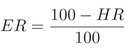
Here, F M R and F N M R are the False Match Rate and False Non Match Rate of a system, respectively. The F M R and F N M R are calculated from the genuine and imposter score distribution. In Eq. (4.20) and (4.21), N is the number of samples in the database, PR is the penetration rate of the indexing system and ER is the indexing error. The ER is calculated using Eq. (4.22) where HR represents the hit rate of the indexing technique.
4.7.2 Databases
In this experiment, five different iris image databases are used: Bath University Iris Database (BATH) [1], CASIA-IrisV3-Interval Iris Database (CASIAV3I) [2], CASIA-IrisV4-Thousand Iris Database (CASIA-V4T) [3], Multimedia University Iris Database Version-2 (MMU2) [4] and West Virginia University Iris Database Release 1 (WVU) [5]. A detailed description of each database is given in the following.
Bath University Iris Database (BATH): The BATH database [1] contains 1000 eye images of 25 persons. Each person has 20 images of left eyes and 20 images of right eyes. These images are high resolution (1280×960 pixels), and have been compressed with JPEG-2000 to 0.5 bits/pixel. The database is created in conjunction with the University of Bath and Smart Sensors Limited. It may be noted that the iris data of left and right eyes of a person are different [9], therefore, 50 unique subjects are considered in BATH database.
CASIA-IrisV3-Interval Iris Database (CASIAV3I): CASIAV3I database [2] is collected by the Institute of Automation at the Chinese Academy of Sciences (CASIA). This database contains 2639 eye images of 249 persons. The eye images in the database are captured from 395 eyes. The iris images are captured with the close-up iris camera developed by Center for Biometrics and Security Research (CBSR). The most of the images are taken in two sessions, with at least one month interval in indoor environment. The resolution of image is 640×480 pixels. From the CASIAV3I database 395 unique subjects are considered as the two eyes are different for a person.
CASIA-IrisV4-Thousand Iris Database (CASIAV4T): This database is also developed Institute of Automation at the Chinese Academy of Sciences [3]. The CASIAV4T database contains 200000 eye images of 1000 persons and each person has 10 left and 10 right eye images. All iris images are 640×480 pixels resolution and collected under near infrared illumination using IKEMB-100 camera. A total of 2000 unique subjects are considered for the CASIAV4T database.
Multimedia University Iris Database Version-2 (MMU2): The MMU2 database is collected at Multimedia University [4]. It contains 995 eye images from 100 persons. Five images are captured from each eye of a person. There are 5 left eye images which are excluded from the database due to cataract disease. The images are captured using Panasonic BM-ET100US camera and with 320×238 resolution. The total number of unique subjects considered for this database is 199.
West Virginia University Iris Database (WVU): This database is created by Center for Identification Technology Research, West Virginia University [5]. The database contains 3099 eye images from 244 persons. Left and right eye images are captured from 241 and 236 persons, respectively. In the WVU database, one to twenty samples are captured for each eye. The images are captured using OKI IRISPASS-H handheld device with 480×640 pixels resolution. Total 477 unique subjects are considered from WVU database in our experiment.
A summary of all the databases is given in Table 4.1.
4.7.3 Evaluation Setup
To evaluate the performance of the proposed approach, all samples of all virtual users are divided into two sets: Gallery and Probe. The samples in the Gallery are enrolled into the index database and samples in the Probe are used as query to search the index database. The 80% samples of each subject are used to create the Gallery and other 20% to create the Probe. The samples of the Gallery Set are selected randomly from each subject.
Table 4.1: Characteristics of databases used in our experiments

The experiments are done with an Intel Core2Duo processor (2.00 GHz) and 2.0-GB memory. GNU Compiler Collection (GCC) 4.3 compiler is used to develop compile the program.
4.7.4 Validation of the Parameter Values
The experiments are involved with different parameters and resources. Eventually, the reported experimental results are subjected to the validity of the above resources and assumptions on values of parameters. In the following, the values of different parameters are validated.
The validity [20] is assessed on the basis of experimental evaluation of the variables. In the experiment, three parameters namely number of scales (S), number of orientations (K) and δ are considered. First, the assumed values of number of scales and number of orientations of Gabor filter are validated. Next, the value of δ is validated.
4.7.4.1 Values of S and K
In the experiment, the number of scales (S) and orientations (K) for feature extraction are decided so that it should give better results. It may be noted that if the number of scales and number of orientations increase, then the number of features in index key increases. On the other hand, the memory requirement to store the index keys also increases when the number of features in index key increases. Further, HR increases as the number of features increases. Hence, there is a trade-off between the number of scales and orientations (and hence memory overhead) with the HR. The experimentation is done with different scales and orientations, and the result on the CASIAV3I database is shown in Fig. 4.6. In this experiment, 10 different scales and 10 different orientations are considered. Figure 4.6(a) and (b) show the H R and P R for different combination of scales and orientations, respectively. It is observed that a higher number of scales and orientations gives the good HR but this also gives high P R which is not desirable. On the other hand, small values of number of scales and orientations give good P R but it give poor HR which is also not desirable. From Fig. 4.6, it is observed that the HR does not change significantly when the number of scales and orientations are increased beyond 3 and 4, respectively. Again, from Eq. (4.23), it is observed that the memory requirement to store the indexed features is directly proportional to the number of features used in indexing. In other words, with large values of number of scales and orientations memory requirement increases greatly without much improvement in H R. With this observation the value of scale is chosen as 3 and orientation is chosen as 4. In fact, this combination gives a better HR and P R as shown in Fig. 4.6.

Figure 4.6: HR and P R with different scales and orientations.
4.7.4.2 Value of δ
To decide the value of δ, HR and P R are calculated for the different values of δ. Figure 4.7 shows the result for different values of δ. From Fig. 4.7(a), it is observed that the HR does not increase significantly beyond the value of δ = 5. On the other hand, from Fig. 4.7(b), it is observed that PR is changing rapidly after δ = 5. Considering this trend it is appropriate to set the value of δ as 5.
4.7.5 Evaluation
The efficiency of the iris indexing technique is judged with respect to accuracy, searching time and memory requirement. The experimentations are done with the gallery and probe sets created in Section 4.7.3.
4.7.5.1 Accuracy
In this experiment, the best match for each sample in the Probe set at the first rank is analyzed. The rank one HR, P R and retrieving time are calculated to measure the accuracy. The results are summarized in Table 4.2. From Table 4.2, it is observed that the HR for WVU is considerably less because the quality of the iris images in WVU database are poor than the other databases. It may be noted that the average P R of BATH, CASIAV3I|indexCASIAV3I, CASIAV4T, MMU2 and WVU iris databases are 11.6%, 15.3%, 16.9%, 14.3% and 10.8%, respectively. From Table 4.2, it is observed that the retrieving time in CASIAV4T is slightly higher than the other databases though the size of database is significantly larger than others.

Figure 4.7: HR and P R for different values of δ.
The result is also substantiated in terms of CM S which gives the probability of at least one correct identity is present within a top rank. How C M S varies with rank is shown in Fig. 4.8 as CMC curve. It is obvious that CMS increases with the increase of rank. From Fig. 4.8, it is observed that 99.4%, 98.8%, 98,7, 98.9% and 98.8% C M Ss are possible within top 60 ranks for BATH, CASIAV3I, CASIAV4T, MMU2 and WVU databases, respectively. In the existing literature on iris indexing, the best reported result [24] so far is 98.56% C M S within top 100 rank for CASIAV3I iris database. In other words, if top 100 rank is considered in this approach then the CMS will eventually increase.
Table 4.2: H R and P R for different iris image databases


Figure 4.8: C M C curves with reference to different databases.
Further, the performance of this method is analyzed with respect to F P I R and F N I R on CASIAV3I database. To do this, first F M R and FNMR are calculated as follows. Each query template of the Probe set is matched with each template in the Gallery set using Daugman’s [11] iris recognition method. In this experiment, 3,000 genuine pairs and 1,242,608 imposter pairs are considered from the Gallery and Probe of CASIAV3I database. Then, the genuine score and imposter score are calculated using Daugman’s method [11] for each genuine and imposter pairs, respectively. Finally, FNIR and FPIR are calculated for an identification system [22] without indexing and with indexing using Eq. (4.20) and (4.21), respectively. The trade-off between F P I R and F N IR for the identification system without indexing and with indexing is shown in Fig. 4.9 for CASIAV3I iris database. From the experimental results, it may be interpreted that 0.72% F P IR and 3.95% F N IR can be achieved with indexing and 3.93% F P I R and 3.83% F N I R without indexing. From Fig. 4.9, it is observed that using this indexing approach low F P IR for an F N IR can be achieved.

Figure 4.9: F P I R vs. F N I R curves with and without indexing for CASIA-V3-Interval database.
4.7.5.2 Searching Time
The run-time complexity is analyzed with big-O notation for gallery match corresponding to a query sample. Let N be the total number of samples enrolled in the database (from P number of subjects), and each subject has Q number of samples. With reference to the Algorithm 4.3, given a query template, the identities of subjects (IDL) and median values (M D L) stored at TabIndex position are retrieved from the ith(i = 1, 2,..., 12) table (Tablei). TabIndex is calculated using Eq. (4.17). The time complexity of this process is O(1). Next, the IDL sets are retrieved corresponding to the values min(M DL) − δ to max(M DL) + δ from Tablei and added these names to Si for rank calculation. This process can be accomplished in O(1) time. Let IL be the average size of the IDL list. The rank calculation process can be done in O(I L) time. In the worst case, when all samples are stored in one position then I L is equal to N , which is very unlikely to occur.
The search efficiency is analyzed by measuring the average time taken to retrieve iris templates from the database for a given query iris. Let tp be the average time to perform addition, subtraction and assignment operations. This indexing approach requires 6 comparisons to retrieve candidates corresponding to one feature and a candidate set of size I L is retrieved using 12 features (see Algorithm 4.3). Therefore, the time taken (Tr ) to retrieve a candidate set of size I L is (tp ×6)×12. Let td be the time to compare query iris template with one stored iris template for matching. Hence, the search time using this indexing approach (Ts) is Tr + td × IL. On the other hand, linear search requires td × N time. Thus, this indexing approach takes less time than the linear search approach because I L << N .
The result for each approach is summarized in Table 4.3. It is observed that, on an average, 52% less time is required to search the database with the this indexing compared to the non-indexed search.
Table 4.3: Time required (in second) to retrieve best match using indexing and without indexing

4.7.5.3 Memory Requirement
This indexing approach considers a number of tables to index iris data. In this experiment, the amount of memory overhead for the indexing mechanism is analyzed. In the indexed database, each table stores a sample one time and each table has entries for all samples. Each entry requires 4 bytes. Hence, the memory requirement to store all index keys is calculated using Eq. (4.23).
In Eq. (4.23), Tsize denotes the size of a table, L is the number of features used for indexing, N is the number of samples in the database and B is the memory required to store a sample. Figure 4.10 shows the average table size and memory requirement to store the different number of samples for different databases. From Fig. 4.10(a), it can be shown that the table size does not vary linearly when the number of enrolled samples increases. Further, Fig. 4.10(b) shows that the memory requirement to store samples is increased linearly. This result substantiates that the total memory is not increasing non-polynomially.
The memory cost for 1,000,000 and 1,000,000,000 subjects are calculated according to Eq. (4.23). The size of a table depends on the range of values of Gabor energy features. From Fig. 4.10(a), it is observed that the size of a table is approximately 1.2 times the number of samples (according to our experiment with 1,000 enrollments). It may be noted that beyond 1,000 enrollments the size of the table does not increase significantly. For a large number of enrollments, it may be assumed the size of the table as 1.5 times the number of subjects. Further, it is assumed that 4 bytes are required to store an identity of a sample for a subject. With this consideration, the memory requirement for 1,000,000 and 1,000,000,000 enrollments are estimated as follows.

Figure 4.10: Average table size and memory requirements to enroll the iris data for different iris image databases.

Hence, to store the above mention data this approach requires approximately 115MB and 112GB storage, respectively.
4.8 Comparison with Existing Work
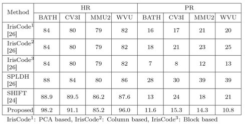
This work is compared with some of the existing indexing techniques mentioned in [26, 24]. To compare this approach the top five matches are considered for all databases. Note that existing approaches do not follow rank-based evaluation. Hence, the result of the existing work are compared with the same at fifth rank of this algorithm with respect to HR and P R. The fifth rank in this approach is considered because in all databases minimum five samples of a subject are present. Table 4.4 shows the comparison results. From Table 4.4, it is observed see that this approach gives better H R than the approaches proposed in [26, 24]. It may be noted that the penetration rate according to this approach is comparable to the existing indexing techniques.
The existing algorithms are also analyzed to compare the retrieval times. In indexing method, a set of templates is retrieved for a given query and then searching or matching is performed on the retrieved data. The efficiency of indexing system can be measured in terms of the retrieval time. The retrieval times of existing techniques are also analyzed as follows. The IrisCode based method [26, 25] stores iris data into a number of clusters using k-means clustering. For a given query sample, the IrisCode method determines the target cluster for closest match. This indicates that the query template is needed to compare with all cluster centers to find a matched cluster. This technique requires minimum K number of comparisons to find the appropriate cluster where K is the number of clusters. Typical values of K = 5, 10, 15, 20 for 2000 samples and K may increase when the number of enrolled samples increase. Hence, IrisCode based technique requires K number of O(1) computations to retrieve similar iris templates. It also may be noted that the number of K varies with the sizes of databases [26, 25].
Table 4.4: Comparison of HR and P R with existing work
The SPLDH based approach [26] uses tree data structure to store iris data. The minimum search time for tree data structure to find a match with query template is O(logN ) which is the height of the tree with N number of enrollments. This is so because the height of the tree depends on the number of samples stored in the tree.
The SIFT based technique [24] uses geometric hashing for indexing. In SIFT based indexing, minimum M number of comparisons are required to hash all key points where M is the number of key points in query sample and the value of M is approximately 100. This time is independent of the sizes of databases.
On the other hand, in the proposed approach, the similar templates are retrieved corresponding to twelve index key values of query. This requires twelve comparisons in O(1) time. Further, the retrieval time of proposed algorithm does not depend on the sizes of the databases. The retrieval time complexities and execution times (specific to computing environment Intel Core 2, 2.0GHz processor, 2 GB Memory) of different indexing mechanisms are summarized in Table 4.5.
4.9 Summary
A novel indexing technique is proposed using Gabor wavelet features. The proposed technique requires a less number of features compared to the existing approaches. As a consequence, it requires less memory to store index data. Further, with less number of features, the index space is organized in such a way that a set of identities are retrieved similar to the query in a constant time. The memory and computation time advantages are achieved without compromising the accuracy. In the proposed approach, approximately 99% CMS can be achieved. Finally, the work has been published in [15]
Table 4.5: Retrieval time complexity and execution time of different indexing mechanisms
| Indexing method | Retrieval time complexity | Time (ms) |
|---|---|---|
| IrisCode (row/column/ block based averaging, PCA) | O(1) | 0.02 |
| Minimum K comparisons are required where K is the number of clusters (typically K = 5, 10, 15, 20 for 2000 samples and the value of K increases as the number of enrollments increases). | ||
| SPLDH | O(logN) | 64 |
| Execution time depends on the number of enrolled samples (N ). | ||
| SIFT | O(1) | 231 |
| Minimum M comparisons are required where M is the number of key points in an iris image. Typical value of key points is ≈100. | ||
| Proposed approach | O(1) | 0.014 |
| Only FL comparisons are needed where FL is the dimension of the index key. In our approach FL = 12 and it is independent of the number of samples. |
Bibliography
- [1] Bath Iris. University of Bath Iris Image Database. URL http://www.bath.ac.uk/elec-eng/research/sipg/irisweb/index.html . (Accessed on August, 2008).
- [2] CASIA Iris Database. CASIA-IrisV3-Interval, . URL http://www.cbsr.ia.ac.cn/IrisDatabase.htm. (Accessed on September, 2010).
- [3] CASIA Iris Database. CASIA-IrisV4-Thousand, . URL http://www.cbsr.ia.ac.cn/IrisDatabase.htm. (Accessed on March, 2012).
- [4] MMU2. Multimedia University: MMU2 Iris Image Database. URL http://pesona.mmu.edu.my/~ccteo/. (Accessed on November, 2008).
- [5] WVU Iris Database. Multimodal Biometric Dataset Collection, BIOMDATA, Release 1,. URL http://citer.wvu.edu/multimodal_biometric_dataset_collection_biomdata_release1 . (Accessed on September, 2010).
- [6] B. Bhanu and X. Tan. Fingerprint Indexing Bsed on Novel Features of Minutiae Triplets. IEEE Transactions on Pattern Analysis and Machine Intelligence, 25(5):616–622, 2003. ISSN 0162-8828.
- [7] R. Cappelli, M. Ferrara, and D. Maltoni. Fingerprint Indexing Based on Minutia Cylinder-Code. IEEE Transactions on Pattern Analysis and Machine Intelligence, 33(5):1051–1057, 2011.
- [8] J. Daugman. Uncertainty Relation for Resolution in Space, Spatial Frequency, and Orientation Optimized by Two-dimensional Visual Cortical Filters. Journal of The Optical Society of America , 2(7):1160–1169, 1985.
- [9] J. Daugman. Biometric Personal Identification System Based on Iris Analysis, 1994.
- [10] J. G. Daugman. Complete Discrete 2d Gabor Transforms by Neural Networks for Iimage Analysis and Compression. IEEE Transactions on Acoustics, Speech, and Signal Processing, 36(7): 1169–1179, 1988. doi: http://dx.doi.org/10.1109/29.1644.
- [11] J. G. Daugman. High Confidence Visual Recognition of Persons by a Test of Statistical Independence. IEEE Transactions on Pattern Analysis and Machine Intelligence, 15(11):1148–1161, November 1993.
- [12] S. Dey and D. Samanta. An Efficient Approach to Iris Detection for Iris Biometric Processing. International Journal of Computer Applications in Technology, 35(1):2–9, 2009.
- [13] S. Dey and D. Samanta. An Efficient and Accurate Pupil Detection Method for Iris Biometric Processing. International Journal of Computers and Applications, 32(2):141–148, 2010.
- [14] S. Dey and D. Samanta. Fast and Accurate Personal identification based on Iris Biometric. International Journal of Biometrics, 2 (3):250–281, June 2010.
- [15] S. Dey and D. Samanta. Iris Data Indexing Method using Gabor Energy Features. IEEE Transactions on Information Forensics and Security, 7(4):1192–1203, 2012.
- [16] D. Gabor. Theory of Communication. Journal of the Institution of Electrical Engineers - Part III: Radio and Communication Engineering , 93(26):429–457, 1946.
- [17] R. C. Gonzalez and R. E. Woods. Digital Image Processing. Prentice Hall, 2nd edition, 2002.
- [18] Aglika Gyaourova and Arun Ross. Index Codes for Multibiometric Pattern Retrieval. IEEE Transactions on Information Forensics and Security, 7(2):518–529, 2012.
- [19] J. Han and K.-K. Ma. Rotation-invariant and Scale-invariant Gabor Features for Texture Image Retrieval. Image and Vision Computing, 25(9):1474–1481, 2007. doi: http://dx.doi.org/10.1016/j.imavis.2006.12.015 .
- [20] B. A. Kitchenham, S. L. Pfleeger, D. C. Hoaglin, and J. Rosenberg. Preliminary Guidelines for Empirical Research in Software Engineering. IEEE Transactions on Software Engineering, 28(8): 721–734, 2002.
- [21] L. Ma, T. Tan, Y. Wang, and D. Zhang. Personal Identification based on Iris Texture Analysis. IEEE Transaction on Pattern Analysis and Machine Intelligence, 25(12):1519–1533, 2003.
- [22] D. Maltoni, D. Maio, A. K. Jain, and S. Prabhakar. Handbook of Fingerprint Recognition. Springer, London, 2nd edition, 2009.
- [23] B. S. Manjunath and W. Y. Ma. Texture Features for Browsing and Retrieval of Image Data. IEEE Transactions on Pattern Analysis and Machine Intelligence, 18(8):837–842, 1996. doi: http://dx.doi.org/10.1109/34.531803.
- [24] H. Mehrotraa, B. Majhia, and P. Gupta. Robust Iris Indexing Scheme using Geometric Hashing of SIFT Keypoints. Journal of Network and Computer Applications, 33(3):300–313, 2010. doi: http://dx.doi.org/10.1016/j.jnca.2009.12.005.
- [25] R. Mukherjee. Indexing Techniques for Fingerprint and Iris Databases. Master’s thesis, College of Engineering and Mineral Resources at West Virginia University, 2007.
- [26] R. Mukherjee and A. Ross. Indexing Iris Images. In Proceedings of the 19th International Conference on Pattern Recognition , pages 1–4, Tampa, Florida, USA, December 2008. ISBN 9781424421756. doi: http://dx.doi.org/10.1109/ICPR.2008.4761880.
- [27] N. B. Puhan and N. Sudha. A Novel Iris Database Indexing Method using the Iris Color. In Proceedings of the 3rd IEEE Conference on Industrial Electronics and Applications (ICIEA 2008), pages 1886–1891, Singapore, June 2008. doi: http://dx.doi.org/10.1109/ICIEA.2008.4582847 .