Chapter 6: One-Sample Tests
Performing a One-Sample t Test
Nonparametric One-sample Tests
Introduction
SAS Studio comes equipped with statistical tasks for just about any statistical query that you will need as a student or researcher.
You may have very little need to perform a one-sample test (of any kind), but let's start here anyway. First, this will show you how to navigate the various tabs that are common to all the statistical tasks. You will also see how to test some basic assumptions that need to be met before performing most parametric tests.
Performing a One-Sample t Test
A one-sample test is usually used when you have a null hypothesis that the mean of a sample is equal to a predetermined value. For example, suppose that you have several years of data on the weight of perch in a particular location. You wonder if the mean weight of these fish in the current season is different (perhaps lighter) from the mean weight computed from thousands of fish taken in the past several years.
For this imaginary situation, suppose that the mean weight of perch in your location, determined over several years, is 500 grams. You take a sample of the next 56 perch that are caught in this location and put the data into an Excel spreadsheet (called Perch.xlsx) as shown in Figure 1 below:
Figure 1: Perch Data in the File Perch.xlsx

Notice that the worksheet also contains the height and width of each fish. (You may want to work with these variables later.)
To perform a one-sample t test, your first step is to convert the Excel Workbook into a SAS data set. To make things simple, you placed the Perch.xlsx workbook in c:SASUniversityEditionmyfolders, the location that was mapped to a location on your virtual machine called 'myfolders' when you installed SAS University Edition.
You use the Import Utility to import this data set. The steps are as follows:
1. Select the Tasks and Utilities tab and expand the Utilities options: It looks like this:
Figure 2: Expand the Utilities Options

Double-click Import Data to see the screen below:
Figure 3: Select Import Data
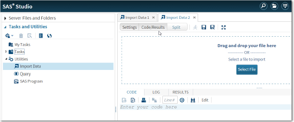
Remember, you can either click Select File or you can open the Server Files and Folders tab, locate the file Perch.xlsx, and drag it to the Drag and drop area. Because you used the Select File option in an earlier example, let's find the workbook under My folders and drag it over. It looks like this:
Figure 4: Using the Server Files and Folders Tab

Place the cursor on Perch.xlsx, hold down the left mouse button, and drag it to the Drop and drag area. You decide to name the SAS data set Perch and place it in the Work library. You do this by clicking the Change button under the Output Data section of the screen (as shown in Figure 5 below):
Figure 5: Use the Change Button to Name the Output Data Set and Place it in the Work Library

Make sure that the box next to Generate SAS variable names is checked (this is the default). This uses the column names from the spreadsheet to create SAS column names.
You are now ready to test if the mean weight of your 56 perch is different from the historical mean (that you can consider a population value) of 500. To start, select Tasks and Utilities ▶ Statistics ▶ t Tests,
Double-clicking t Tests brings up the following screen:
Figure 6: t Test Statistical Task

Select Work.Perch as the data set and make sure that One-sample test is selected in the Roles menu (this should be the first item in the pull-down list). Above the Analysis variable box, click the plus sign to bring up a list of numeric variables from the Perch data set. You will see Weight, Height, and Width listed. You can click Weight and then click OK or just double-click Weight. In either case, you will see Weight listed as the analysis variable.
Next, click the Options tab. This brings up the following:
Figure 7: Options for t Test
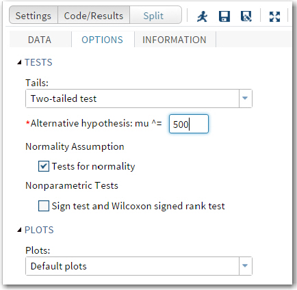
You select Two-tailed test and specify the alternative hypotheses as mu (µ) not equal to 500. You may be more familiar with stating that the null hypothesis is µ = 500 instead of the alternative hypothesis, but they are equivalent. Finally, check the box for Tests of normality and click the Run icon.
Figure 8: First Section of the One-sample t Test

Figure 8 shows several methods for testing the null hypothesis that the distribution (of Weight in this example) is normally distributed. All of these tests reject the null hypothesis (at the α = .05 level). One of the assumptions for one- or two-sample t tests is that the data values come from a population of values that are normally distributed. At this point, you may be tempted to abandon the t test and choose a nonparametric alternative such as a sign test or a Wilcoxon rank sum test.
The decision whether to use a parametric test should not be determined solely by these tests of normality. You may recall that the central limit theorem states that the sampling distribution will be normally distributed, regardless of the population distribution, providing that n (the sample size) is sufficiently large. A sample size that is considered sufficiently large depends on the shape of the distribution of values. If the distribution is somewhat symmetrical, sufficiently large may be quite small (10 or 20). If the distribution is highly skewed, sufficiently large may be quite large. Before you decide to abandon the one-sample t test, you should take a look at the distribution of weights. The one-sample t test task produces both a histogram and a Q-Q plot to help you understand how your data values are distributed.
Figure 9, part of the output from the one-sample t test, shows a histogram with a normal distribution and a kernel distribution (a piecewise, smooth fit to the data) superimposed. Below the histogram, you also see a box plot. Although this is a skewed distribution, you may decide that with a sample size of 56, you can rely on the t test to decide if you should accept the alternative hypothesis (reject the null hypothesis). You probably want to check the nonparametric test results as well (you will see this later in this chapter).
Figure 9: Histogram and Box-Plot for Weight

Another way to investigate deviations from a normal distribution is displayed in a Q-Q plot shown in Figure 10:
Figure 10: Q-Q Plot for Weight

A Q-Q plot (stands for Quantile-Quantile) plot shows quantile values (think of these as z-values) on the x-axis and weight values on the y-axis. The closer the data points lie to the straight line on the plot, the closer the data values represent a normal distribution.
Let's go back and look at the results of the one-sample t test.
Figure 11: One-sample t Test results

The mean weight of your 56 perch was 382.2 with a standard deviation of 347.6. The 95% confidence limits (labeled 95% CL Mean in the output) indicate that you are 95% confident that the population mean from which you drew your sample is between these two values (289.1 and 475.3). Notice that the value 500 is not in this interval. Finally, you see a t value of -2.54 with a probability of .0141. If you set your α level at .05, you can now reject the null hypothesis and state that you believe that perch weights are lower than the historical value of 500.
Nonparametric One-sample Tests
Because the distribution of weights is significantly different from a normal distribution, you decide it would be a good idea to perform some nonparametric tests to confirm the conclusion from the one-sample t test. All you need to do is go back to the Options tab and request nonparametric tests. Because you have already run tests for normality and produced plots, you can uncheck the box next to Tests for normality and, in the menu for plots, select Suppress all plots. A portion of the Options screen is shown in Figure 12:
Figure 12: Option to Compute Nonparametric Tests

Click the Run icon to obtain the following:
Figure 13: Output from Nonparametric Tests
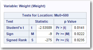
The same t table as shown in Figure 11 is produced (not shown) along with two nonparametric tests—the sign test and the signed rank test (the full name is the Wilcoxon Signed Rank test). Both of these tests produced p-values less than .05, backing up your conclusion based on the t test.
Conclusions
One of the advantages of running SAS Studio is the ease with which you can perform a large number of statistical tests. Yes, you still need to understand which tests to run and verify that the assumptions for those tests are satisfied. But once you have done this, getting your results is a few mouse clicks away.
Problems
6-1: Using the workbook Diabetes.xls, create a temporary SAS data set called Diabetes. Next, conduct a one-sample t test with the null hypothesis of Glucose = 200 (alternate hypothesis Glucose not equal 200). Include tests for normality and nonparametric tests.
6-2: Using the SASHELP data set Fish, test if the mean weight of Perch is equal to 500. To do this, click Filter on the Data tab and use the expression:
Species = 'Perch'
Include test for normality as well as histograms and Q-Q plots. After looking at these tests and plots, rerun the t test task requesting a Wilcoxon Rank sum test.
6-3: Using the SASHELP data set Heart, test if the mean weight is equal to 150. Include a test for normality and make sure that default plots is selected. Can you explain why the test is so highly significant when the mean weight is 153.1?