Chapter 11: Simple and Multiple Regression
Describing Simple Linear Regression
Understanding the Diagnostic Plots
Demonstrating Multiple Regression
Demonstrating Stepwise Multiple Regression
Introduction
Correlation analysis identifies relationships between variables—regression analysis allows you to predict one variable based on values of another variable (simple regression) or a combination of variables (multiple regression).
The concept behind simple or multiple regression is to select one or more variables (sometimes called predictor variables) that can be combined to predict an outcome (dependent variable). The models described in this book are all linear models.
There are several reasons why regression techniques are useful. One reason is that we can use the resulting regression equation to predict a value. For example, given the gender, height, and weight of a person, you could predict the maximum lung volume for that person. Another reason why regression is used is to help explain the relation among a set of variables. That is, we can look at the influence of one or more variables to better understand the nature of a dependent variable. If more than one predictor variable is used, the analysis looks at all predictor variables simultaneously.
Regression, especially multiple regression, needs to be done carefully. There are a number of diagnostic plots produced by the regression task that are useful in deciding if the assumptions for regression are met by your data. In addition, you can test for influential data points (data values that can change the results of the analysis if they are included or not), and test for multi-collinearity (predictor variables correlated with each other). Including highly correlated predictor variables in a multiple regression can lead to strange and paradoxical results.
Describing Simple Linear Regression
Let's use the permanent SAS data set Exercise, described in the last chapter to demonstrate simple (that is, single predictor variable) linear regression. Intuition (plus the correlation matrix produced in the last chapter) tells you that there should be a positive relationship between a person's resting heart rate and this person's pulse rate while running. To run a regression on these two variables, call up the Linear regression task:
Tasks and Utilities ▶ Statistics ▶ Linear regression
It looks like this:
Figure 1: Select Data Source and Specify Variables

You see that the Exercise data set, located in the BOOKDATA library is selected in the Data field; Run_Pulse is selected as the dependent variable and Rest_Pulse is selected as a continuous (independent) variable.
The next step is to specify your model. Click the Model tab to do this:
Figure 2: Specify the Model

First, click Edit and then highlight Rest_Pulse in the Variables list. Next, click Add to add this variable to the model. In the box labeled Model effects, you now see the intercept and Rest_Pulse listed. Click OK to continue.
The last step, before running the model, is to click Options. This tab allows you to select additional statistics and plots:
Figure 3: Specify Plots

Select Diagnostic plots and Residuals for each explanatory variable. You can request the residual plots as a panel of plots or individual plots. For most situations, a panel of plots is sufficient. (Note: The diagnostic plots shown in this chapter are actually selected from individual plots.)
It's time to run the model. The first section of output is the ANOVA table shown in Figure 4:
Figure 4: Regression Results

Because the number of observations read and used are equal (with a value of 50), you know that there were no missing values for the variables Rest_Pulse and Run_Pulse. The mean square due to the model is much larger than the mean square due to error, yielding a very large F-value and a low p-value. The mean of the dependent variable (Run_Pulse) is 112.92, and the R-square is .5710. The linear regression task also computes an adjusted R-square. This value is useful when you have several independent variables in the model. The addition of independent variables in a model causes the value of R-square to increase even if independent variables are only randomly correlated with the dependent variable. The value labeled Adj R-Sq adjusts for the number of independent variables in your model and is a way to compare models with different numbers of independent variables.
The next section of the output (Figure 5) shows the intercept and slope of the regression line:
Figure 5: Parameter Estimates

You are not interested in the value of the intercept, except in estimating value of Run_Pulse. (The intercept would be the value of Run_Pulse for a Rest_Pulse of 0, a condition requiring immediate medical attention.) The parameter estimate for Rest_Pulse (.73297) is the slope of the regression line. To compute a value of Run_Pulse for any given value of Rest_Pulse, use this equation:
Run_Pulse = 63.15163 + .73297*Rest_Pulse
Figure 6 shows the actual data points, the regression line, and two types of confidence limits.
Figure 6: Regression Line, Confidence Limits, and Sources of Variation

To help explain the two sources of variation in a simple linear model, a single data point was selected (located in the upper-right side of the plot). The horizontal line on the plot is the mean of Run_Pulse for the total sample (it is 112.92). The selected data point contributes to the total sum of squares for two reasons. First, given a value of Rest_Pulse equal to about 85 (the value of Rest_Pulse for the selected point), you would expect a Run_Pulse value of about 125 (the value that lies on the regression line). The difference between the mean Run_Pulse and the point on the regression line represents the amount that the regression contributes to the sum of squares for this particular point. The difference between the regression line and each data point (called a residual) contributes to the error sum of squares. If all the data points were close to the regression line, most of the contributions to the sum of squares would be due to the regression, and a smaller portion would be due to error, indicating a good fit.
The shaded portion of this graph represents the 95% confidence limit for the prediction of Run_Pulse for any given value of Rest_Pulse. The other, much wider confidence limits are for individual data points. Given a value of Rest_Pulse, you are 95% confident that a random data point will be within these limits.
Understanding the Diagnostic Plots
Before you start interpreting the relatively high R-square and the low p-value for this model, you need to look at some diagnostic plots to determine if the residuals are normally distributed and if the variance of the residuals seems homogeneous across different values of Rest_Pulse. These are two assumptions behind linear regression. It's time to inspect some of the diagnostic plots:
Figure 7 is one of the diagnostic plots produced by the regression task. It shows the difference between the actual value of Run_Pulse and the value predicted by the regression.
Figure 7: Residual Plot

There are several things to notice in this plot. First, the points seem mostly random. If you saw a pattern in these points (such as the points curving up or down), you might suspect that a non-linear component could improve the model. Next, the spread of the points around 0 does not tend to increase or decrease with different values of Run_Pulse. To inspect the distribution of the residuals, you can inspect the Q-Q plot (Figure 8), included as one of the diagnostic plots.
Figure 8: Q-Q Plot of the Residuals

Notice that the points on this plot fall very closely around the straight line. This demonstrates that the assumption that the residuals are normally distributed is satisfied.
The last plot that is discussed here shows Cook's D for values of Run_Pulse.
Figure 9: Cook's D for Run_Pulse

Cook's D is a measure of influence for each data point. There are several measures of influence available in the regression task. They all involve running the regression with and without each data point removed to see if the removal of a particular data point changes either the predicted value or the betas (coefficients) in the regression equation. Cook's D measures changes in the predicted value when a data point is removed. Large values for Cook's D indicate these points are influential. If you place your cursor on one of these large values (see the hand pointer on the plot) the ID for that data point is displayed. You may want to check that this data point is a valid data point and not the result of a data error.
Demonstrating Multiple Regression
Multiple regression, as the name implies, uses more than one predictor variable to estimate a single dependent variable. You can use the same Exercise data set used in the simple linear regression section to see how to run a multiple regression using SAS Studio. A useful first step is to use the Correlation task to produce a correlation matrix for all the variables of interest. The next two figures are screen shots of the correlation matrix and the scatter plot matrix when the variables Age, Pushups, Rest_Pulse, Run_Pulse, and Max_Pulse are entered as analysis variables. To obtain the scatter plot matrix, the Plot option was selected, and the box labeled "Include histograms" was checked. Here are the results:
Figure 10: Correlation Matrix for the Exercise Data Set

Figure 11: Scatter Plot Matrix for the Exercise Data Set

It is clear from both figures that there are some strong correlations among the variables. The condition where the predictor variables are highly correlated is called multi-collinearity, and it causes serious problems when these variables are all used in multiple regression (as you will see).
So, going on with the demonstration, let's use the variables Age, Pushups, Rest_Pulse, and Max_Pulse to predict Run_Pulse. Select the Linear Regression task; select the BOOKDATA.Exercise data set; and choose Run_Pulse for the dependent variable and all the predictor variables in the box labeled Continuous variables. On the Model tab, select all the variables, click Add, and then click OK.
When you run the task, here is what you will see:
Figure 12: ANOVA Table for Multiple Regression

Notice that the model is highly significant, and the R-square (.8869) and the adjusted R-square (.8768) are fairly large. However, take a look at the parameter estimates (Figure 13):
Figure 13: Parameter Estimates for the Multiple Regression

In the earlier simple regression model, Rest_Pulse was highly significant in predicting Run_Pulse (p < .0001), and the slope (labeled parameter estimate) was positive—here Rest_Pulse is not significant (p = .5221), and the parameter estimate is negative. What's going on?
This result is typical in cases where you have highly correlated predictor variables. You already knew this was the case when you saw the correlation matrix of the variables. This phenomenon is called multi-collinearity. One popular diagnostic test for multi-collinearity is call the VIF. This stands for variance inflation factor. Here's how it works:
If you take each of the predictor variables one at a time and perform a multiple regression with the selected predictor variable as the dependent variable and the remaining predictor variables as independent variables, you will get an R-square for each predictor variable. High values of R-square indicate that a particular predictor variable is correlated with a linear combination of the other predictor variables. Think of it as the degree to which the variable under consideration is more or less already accounted for by the other variables in the regression. Rather than use the R-square values, the VIF is computed as follows:
VIFi=1(1−Ri2)
For example, if an R-square was equal to .9, the VIF would be 1/(1-.9) = 10. Therefore, large values of VIF indicate multi-collinearity problems.
To include the VIF in your regression, click the Options tab, expand the menu next to Display statistics, and select Collinearity. Check the box for Variance inflation factors (Figure 14):
Figure 14: Option for Variance Inflation Factor (VIF)

With this option checked, the parameter estimates table includes the value of the VIF for each predictor variable. Here is the result:
Figure 15; Parameter Estimates with VIF Added

The largest value of VIF is found for Rest_Pulse. The decision of which variables to remove from the regression can be determined by choosing the variables with the highest p-values or highest VIF values. Typically, you take out one variable at a time, rerun the model, and check the VIFs. For this example, Rest_Pulse was removed and the model rerun. See Figure 16:
Figure 16: Model with the Least Significant Variable (Rest_Pulse) Removed

Notice that all the VIFs are low, and the coefficient of Max_Pulse is positive (as it should be). This section should encourage you to check the VIF and inspect a correlation matrix each time you conduct a multiple regression.
This example is a fairly extreme one in that one of the predictor variables has an unusually high simple correlation with the outcome variable, and the independent (predictor) variables tend to be intercorrelated substantially as well. What has been presented here is a purely data-based approach to working with this situation. But in real life, you will almost always want to bring your understanding of the nature of the variables into consideration in analyzing the data. For example, Age is a very different kind of variable from Max_Pulse. And Max_Pulse may be conceptually very close to Run_Pulse. The question of “Just what do I want to explain here?” has to be taken into consideration. But that is a long discussion, and not really the goal of this book. In general, using more than three independent variables, especially ones with a fair amount of intercorrelation, will almost always lead to difficulties in interpretation.
Demonstrating Stepwise Multiple Regression
The final section in this chapter describes several automatic methods for selecting predictor variables in a multiple regression model. Clicking the Selection tab brings up the following screen:
Figure 17: Selection Methods for Multiple Regression

If you leave the default value of None, the regression task will enter all of the predictor variables that you have selected, either as Classification variables or Continuous variables. The other three methods in the list represent automatic selection methods.
Each of these automatic selection methods allows you to choose a criterion for entering or removing variables. The default method is called the Schwarz Bayesian Information Criterion (abbreviated SBC). This method aims to find a model with good predictive properties while limiting the number of predictor variables in the model (called a parsimonious model). Another popular selection method uses the value of R-square or the adjusted R-square to determine which variable to enter or remove from the model.
If you select forward selection as your selection method and R-square as your method to add or remove variables, the program first chooses the variable with the highest R-square value (lowest p-value). It continues to enter the remaining variables based on values of R-square until the p-value for a variable exceeds a default value.
Backward selection is just the opposite—it starts with all the variables in the model and removes them one-by-one until a criterion is met.
One of the most popular selection methods is the last one in the list—stepwise selection. This method is similar to forward selection except that variables already selected may be removed if adding other variables causes a particular variable to no longer satisfy the selection criterion. To demonstrate an automatic selection process, let's use the 25% random sample of birth weights from the SASHELP data set Bweight (first discussed in Chapter 6).
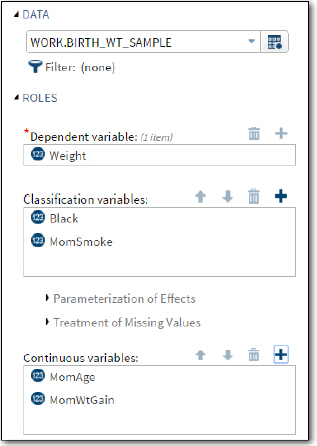
You start this task by selecting the Birth_Wt_Sample data set in the WORK library. The dependent variable is Weight. The two variables Black (1=black, 0=non-black) and MomSmoke (1=yes, 0=no) are selected as classification variables and the two variables MomAge (mother's age) and MomWtGain (mom's weight gain) are selected as continuous variables. (See Figure 18 below):
Figure 18: Choosing Classification and Continuous Variables for Multiple Regression
Click the Selection tab to choose a selection method.
Figure 19: Choosing a Selection Method

For this example, you have chosen stepwise regression and R-square as the add/remove criterion. It's time to run the model. The first section of output shows the selection method and criterion for entering or removing a variable (Figure 20):
Figure 20: Results Showing Selection Method and Select and Stopping Criterion

The next part of the output shows the values for all of your classification variables (Figure 21):
Figure 21: Class Level Information

Now comes the good stuff: The stepwise selection summary shows which variables were entered into the models as well as the order of entry.
Figure 22: Stepwise Selection Summary

All four variables were entered into the model. The last column, labeled Model R-Square, shows the model R-square as each variable is entered into the model.
Important note: The order of entry does not necessarily tell you the relative importance of each variable in predicting the dependent variable. For example, you could have a variable that is highly correlated with the dependent variable but does not enter the model because it was also correlated with other predictor variables that entered first.
One of the default plots shows the value of four different fit methods (Figure 23):
Figure 23: Four Fit Criteria Plots

AIC (Akaike's information criteria – yes, I can't pronounce it either!) and a modified version AICC are displayed in the top two graphs. The stars on the plots indicate that the four-variable model is the "best" model as defined by each criterion. The SBC, discussed earlier, is displayed on the bottom left, and the adjusted R-square is displayed on the bottom right. Although all four criteria selected the same model, this is not always the case.
The familiar regression ANOVA table is shown next.
Figure 24: Regression ANOVA Table

The overall p-value for this model is quite low. However, remember that there are almost 13,000 observations in the 25% random sample, so even small effects can be significant.
A summary of the fit methods is shown in Figure 25:
Figure 25: R-Square, Adjusted R-Square plus other Measures

The last portion of the output shows the parameter estimates along with the t and p-values. Because there are only two levels of the classification variables, they are easy to interpret. For example, the estimate for Black 0 (non-black) is about 218. This means that after all the other variables are adjusted for; babies of a non-black mother are 218 grams heavier than babies where the mother is black. Because smoking is a risk factor for low birth weight babies, you see that if a mother does not smoke (MomSmoke = 0), the babies are almost 253 grams heavier than if the mother smokes.
Figure 26: Parameter Estimates

Conclusions
As demonstrated in the first multiple regression example, failing to pay attention to the diagnostic information, especially multi-collinearity, can result in models that do not make sense. Besides checking the residuals to see if they are approximately normally distributed and that the variance of the residuals is somewhat homogeneous for different values of your independent variables, there is one additional caution: There is a "rule of thumb" that says you should have approximately 10 times the number of observations as predictor variables in your model. If you have too few observations, you may see very high values of R-square that are simply a mathematical fluke and not actual relationships in your model.
You are probably better off to use a rule of thumb that says something more like: 50 observations plus 10 times the number of independent variables. Also, please keep in mind that having a lot of independent variables makes simple interpretation difficult. Less is truly more in most instances in multiple regression. (Thanks to Jeff Smith for adding this insightful paragraph.)
Problems
11-1: Using the data set SASHELP.Heart, run a simple linear regression with Weight as the dependent variable and Height as the independent or predictor variable. Include a scatter plot of the data. Using the parameter estimates, what is the predicted Weight for a person 65 inches tall?
11-2: Using the data set SASHELP.Heart, run a regression with Weight as the dependent variable and Cholesterol, Systolic, and Sex as predictor variables. Include a panel of diagnostic plots. Because this data set contains over 5,000 observations, be sure to increase the default value of 5,000 for the number of data points to plot. Approximately how much lighter is a female than a male with the same systolic blood pressure and cholesterol?
11-3: Using the data set SASHELP.Heart, run a regression with Weight as the dependent variable and Cholesterol, Systolic, Diastolic, and Sex as predictor variables. Add the option to include the VIR and omit all plots. Rerun this same model using stepwise regression. Accept all the defaults for the decision to add or remove effects. Which of the variables are included in the stepwise model?
11-4: Use the Excel workbook Correlate.xlsx to create a temporary SAS data set called Corr. Run a regression on this data set with z as the dependent variable and x and y as continuous predictor variables. Include the option to print the VIR in the output. Notice the parameter estimates for x and y as well as their p-values. It would be instructive to compute a correlation matrix of the three variables x, y, and z using the Correlation analysis task. Return to the regression task and remove y from the model. When you run the model, what can you say about the parameter estimate for x?