Chapter 7: Two-Sample Tests
Unpaired t Test (t Test for Independent Groups)
Nonparametric Two-sample Tests
Introduction
There are two classes of two-sample tests that you will see in this chapter. One is an unpaired t test (also called a t test for independent groups) that is used to compare means between two groups. The other type of two-sample t test is a paired t test. A common situation where a paired t test is performed is when each subject is measured twice, typically before and after some treatment. It can also be used when experimental units are paired on certain characteristics such as gender and age before the experiment and the variable of interest is the difference between values in each pair. Experimental units are often subjects, and that is the terminology subsequently used in the book.
As you saw with the one-sample t test, the two-sample statistical task also performs nonparametric tests, both for paired and unpaired situations.
Unpaired t Test (t Test for Independent Groups)
Let's start by using data from the SASHELP data set called Heart. This data set contains health and demographic information such as gender, health status, height, weight, blood pressure, and many risk factors such as cholesterol and smoking status. Suppose you wish to compare the variable Weight for men and women (variable Sex).
The first step is to open the t Test tab (the same process that you used for the one-sample t test):
Tasks and Utilities▶ Statistics ▶ t Tests (double-click here)
This opens the following screen:
Figure 1: Data Tab for Two-Sample t Test

Data set Heart (in the SASHELP library) has been selected; a Two-sample t test has been selected from the pull-down list; the analysis variable is Weight; and the Group variable is Sex. It is important that the Group variable have only two possible values. If the Group variable has more than two values, you will see an error message in the log.
Before you run the t test, click the Options tab to bring up the following:
Figure 2: Options Tab for Two-Sample t Test

You are selecting a two-tailed test and verifying that the alternative hypothesis is that the two samples come from populations that have different means. For now, check the Tests for normality, leave the Nonparametric Tests unchecked, and accept the Default plots. You are now ready to run the test.
The first section of output is the requested normality tests (one for Females, the other for Males).
Figure 3: Normality Tests for Females and Males

All three tests for females and males show p-values below .05, meaning that you reject the null hypothesis that the distribution of weight for females and males is normally distributed. This is not surprising when you consider that there are over 2000 observations for both females and males. This means that even small deviations from a normal distribution will be significant (the test has high power because of the large sample size). You need to look at the actual distributions to decide if you can use a parametric test to test your hypothesis. The histogram and Q-Q plots appear at the end of the output (shown in Figure 5 and Figure 6).
The next portion of the output contains the means and other statistics on weight for females and males as well as the t- and p-values. This is shown in Figure 4 below:
Figure 4: Two-sample t Table

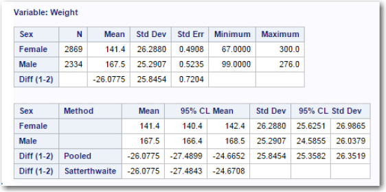
The mean weight for females and males was 141.4 and 167.5 pounds, respectively. The standard deviations were similar (26.2880 and 25.2907). You also see the 95% confidence limits for the means of females and males as well as the mean difference (labeled Diff (1-2)) and the 95% confidence limits for the difference. Note that there are two different confidence limits listed as well as two t- and p-values in the table. One set of values is computed under the assumption that the two groups have equal variance; the other set of values is computed under the assumption of unequal variance.
Which set of values should you use? There are different thoughts on how to approach this issue. The first, and probably the most common strategy, is to look at the F test at the bottom of the figure. The F test tests the equality of variances for the groups. The null hypothesis is that the variances are equal; the alternative hypothesis is that they are not equal. If the p-value for this test is less than .05, you would chose the t- and p- values under the assumption of unequal variances (the method used is labeled Satterthwaite in the table). If the p-value is greater than .05, you would use the values based on equal variances (labeled Pooled in the table).
Another train of thought says to decide before you conduct your study which assumption (equal or unequal variances) you think is reasonable. The idea behind this method is that collecting the data and making the decision based on the same data is somewhat circular. The good news is that for large samples the t test is very robust to the homogeneity of variance assumption, and the two p-values are usually close, even if there are relatively large differences in the variances.
Following rule one in this discussion, you see a p-value of .0503 for the test of homogeneity of variance and decide to use the pooled values in the table. You reject the null hypothesis that the populations from which you took the female and male weight samples have equal means. And you conclude that the female mean was less than the male mean.
Even though the histograms and Q-Q plots are displayed at the bottom of the results, you probably want to look at them before you examine and interpret the t table. These two plots are shown in the next two figures:
Figure 5: Histograms and Box Plots

Figure 6: Q-Q Plots

The histograms look quite close to normal while deviations from normality are a little more obvious in the Q-Q plots. However, with each group having a sample size of over 2000, you feel confident that using a t test is appropriate.
Nonparametric Two-sample Tests
If you want to compare two groups and you feel that the assumptions for a parametric test are not satisfied, the t test statistic task can also perform a Wilcoxon rank sum test, the nonparametric counterpart to the Student's t test.
To demonstrate how this works, let's use the SASHELP data set called Fish to demonstrate the Wilcoxon test. The Fish data set contains weights and several other variables on several species of fish. You decide to compare weights of two species: Roach and Pike. (Note: This author has never heard of a Roach fish.)
This example has two purposes: To demonstrate how to run and interpret a Wilcoxon Rank Sum test and how to filter rows in a table.
You start by double-clicking the t Test task as before. Next, on the Data tab, click Filter (as shown in Figure 7):
Figure 7: Filtering the Fish Table to Select Two Species

This opens the following screen:
Figure 8: Selecting Pike and Roach Species

Type the logical expression as seen in Figure 8. You can type logical expressions in the filter box such as the one to select the two fish species or other logical expressions such as Age < 30 or Height between 54 and 65. For those readers familiar with SQL, you can enter the same types of expressions that you would enter in a WHERE clause, except you do not include the word WHERE in the filter box.
Note: Because Species is a character variable, the values "Pike" and "Roach" must be in single or double quotation marks in the filter expression. For numeric variables, you do not place quotation marks around the numeric values.
You can undo a filter by clicking the small 'x' next to the filter text in the Data window.
You can now click the Run icon to display the results for the test of normality and see histograms for weights of the two selected fish species. The normality test results are shown in Figure 9, and the histograms are displayed in Figure 10.
Figure 9: Test of Normality for Two Species
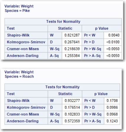
Figure 10: Distributions for Fish Weights

You need to pay closer attention to the distributions of weights because of the much smaller sample sizes for these two fish species (n=20 for Roach and n=17 for Pike). The tests for normality reject the null hypothesis that these weights for Pike come from a population that is normally distributed, and the histograms show a distribution that is not symmetric or normal.
Because of these results, you decide to run a Wilcoxon rank sum test. To do this, simply check the box labeled Wilcoxon Rank Sum Test on the Options tab, as shown in Figure 11:
Figure 11: Requesting the Wilcoxon Rank Sum Test

Because you have already seen the histograms, you can use the menu under Plots to select a Wilcoxon box plot (and deselect the other plots).
Click the Run icon to obtain the following:
Figure 12: Rank Sums for the Wilcoxon Rank Sum Test
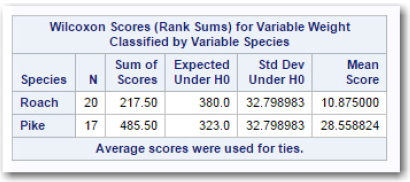
Figure 12 shows the sum of ranks for the two fish species. Here's how it works: You order all the fish weights (both species combined), from lowest to highest, giving then all ranks (the smallest is rank 1, the next smallest is rank 2, etc.). If there are two or more weights that are equal, you give them all the average rank. Finally, you add up the ranks for each species. In the figure above, you see this sum labeled Sum of Scores. If the null hypothesis is true, you would expect the sum of ranks to be about the same for both groups. Looking at the two histograms of weights, you see that, in general, the weights for Roach fish are lighter than the weights of the Pike. Therefore, you expect the sum of ranks for Roach to be lower than the sum of ranks for Pike. If the null hypothesis is true, large differences between the sum of ranks in the two samples are unlikely. That is the basis for computing a p-value for this test.
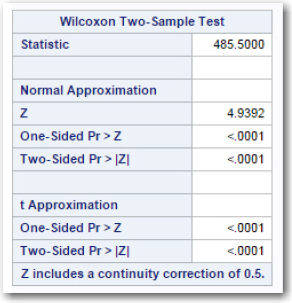
The next portion of the output shows you two ways to compute a p-value. One, useful for larger samples, is a z-test (with a correction for continuity); the other test, sometimes used for smaller samples, is a t approximation. In this table, both p-values are very small, and you can claim that Pike are heavier than Roach based on the population from which the samples were taken.
Figure 13: p-Values for the Wilcoxon Test
Because you checked the box for a Wilcoxon box plot, you are presented with Figure 14:
Figure 14: Distribution of Wilcoxon Scores

This plot shows the distribution of ranks for the two groups of fish. You can see that the Pike weights are given most of the larger rank values.
Paired t Test
The final section of this chapter describes a paired t test. This test is used when the situation either involves two values taken from each subject (such as a score taken before and after a subject is treated) or two subjects who are paired on one or more characteristics. Then one is randomly assigned to one treatment and the second to the other treatment
To demonstrate a paired t test, you can use data from a small study designed to show if a half hour of yoga can lower a subject's heart rate. Ten subjects had their heart rate measured before and after the yoga session, and the results were entered into an Excel workbook called Yoga.xlsx.
This workbook was saved in the folder c:SASUniversityEditionmyfolders. Figure 15 (below) shows the original spreadsheet:
Figure 15: Spreadsheet Containing Before and After Heart Rates

The Import Utility under the Tasks and Utilities tab was used to convert the workbook into a SAS data set called Yoga that was placed in the Work library. The next step is to double-click the t Test tab and enter the appropriate information on the Data tab. The data set name is
WORK.Yoga. A paired t test is selected from the menu, and the two variables, Before and After, are entered as the Group1 and Group 2 variables. (See Figure 16 below.)
Figure 16: Data Tab for Paired t Test

It's time to run the procedure (you are leaving all the defaults on the Options tab). Here are the results:
Figure 17: Test for Normality for Difference Scores

All of the test for normality are not significant. You should not interpret this to mean that the difference scores are normally distributed. With such a small sample (10 subjects), it would take large deviations from a normal distribution to reject the null hypothesis at the .05 level. You will need to look at the histogram (or a Q-Q plot) to help decide if a parametric test is reasonable.
The next section of the output shows the t table. You see that the mean difference is 4.222, the t value is 3.74, and the p-value is .0057. Because the mean difference is positive and the difference score was computed as the before value minus the after value, you can conclude that the yoga session helped reduce heart rate (at the .05 level).
Figure 18: Statistics, t- and p-Values

The final section of the output shows a histogram for the difference scores. Although it doesn't look too much like a normal distribution. It is fairly symmetric and with a sample size of 10, you decide that a t test is appropriate.
Figure 19: Histogram of Difference Scores

If you have any doubts, you should rerun the analysis using a nonparametric test such as the Wilcoxon Signed Rank test. This is accomplished by checking the box on the Options tab that requests this test. (Actually, the option runs both a Sign test and a Wilcoxon Signed Rank test.) Although not shown here, these two nonparametric tests both show a significant difference at the .05 level.
Conclusions
You have seen that the t test statistics task can perform one-sample t tests as well as two-sample paired and unpaired tests. For each of these tests, one or more nonparametric alternatives are provided. Because one of the assumptions for all of the t tests is that the data values are normally distributed (or close to it, depending on the sample size), the task provides you with test of normality as well as histograms and Q-Q plots. One final thought: Do not simply look at the p-values from the normality tests. Doing so often results in incorrect decisions. When sample sizes are large, the tests for normality are often significant. When sample sizes are small, they are rarely significant. And, it is with small samples that deviations from normality are most important.
Problems
7-1: Using the SAS data set Diabetes from problem 6-1, compute a two-sample t test that compares Glucose from two of the three Diet_Drinks values (omit Diet_Drinks = 'Sometimes'). Hint: Your filter statement should read:
Diet_Drinks ne 'Sometimes'
7-2: Using the SAS data set Diabetes from problem 6-1, compute a two-sample t test that compares Glucose between the two values for the variable Insulin (1=yes uses insulin, 0=does not use insulin). Add a test for normality for Glucose.
7-3: (advanced) You have measured the heart rate of 12 subjects before and after they have each drunk a cup of coffee. The values are as follows:
| Coffee and Heart Rate Data | ||||
| Subj | Before | After | ||
| 1 | 74 | 89 | ||
| 2 | 78 | 62 | ||
| 3 | 72 | 77 | ||
| 4 | 70 | 78 | ||
| 5 | 68 | 76 | ||
| 6 | 81 | 79 | ||
| 7 | 55 | 84 | ||
| 8 | 68 | 68 | ||
| 9 | 72 | 82 | ||
| 10 | 61 | 76 | ||
| 11 | 74 | 79 | ||
| 12 | 70 | 79 | ||
Create a SAS data set (call it Coffee) from this data either by entering it into Excel and using the Import utility or by writing a DATA step (if you feel confident in your SAS programming ability). Once you do this, run a paired t test comparing the Before and After values.
7-4: Use the Excel workbook Coffee_HR.xls to create a SAS data set called Coffee_HR. This data set will contain the variables Subj, Group (Coffee or Placebo), and HR (heart rate). Conduct a two-sample t test to compare heart rates between the Coffee and Placebo groups.