Chapter 9: N-Way ANOVA
Performing a Two-Way Analysis of Variance
Interpreting the Two-Way ANOVA Results
Interpreting Models with Significant Interactions
Introduction
You can construct ANOVA models with more than one independent variable. One of the most popular models is called a factorial model. In a factorial model, you compute variances for each independent variable as well as interaction terms. For example, if you want to investigate how race and smoking status affect a baby's birth weight, you could construct a model that looks at race (adjusted for smoking status), smoking status (adjusted for race), and each combination of race and smoking status.
The statistics task N-Way ANOVA helps you analyze factorial models as well as more advanced models that involve crossing and nesting.
Performing a Two-Way Analysis of Variance
One of the data sets in the SASHELP library is called Bweight (stands for birth weight). This fairly large data set contains birth weights for 50,000 babies, along with several variables believed to be related to birth weight, such as race (coded as black or not black), mother's smoking status (smoking or non-smoking), and marital status.
Selecting a Random Sample
Because this is such a large data set, you will see how to take a random subset using one of the Data tasks. In practice, you would use all the data in such a data set, but there are two reasons to consider a subset: First, you will see how to use the Random Subset task; second, using a smaller data set will reduce processing time. (If you are not interested in how to select a random sample, feel free to skip this section and jump right to the two-way ANOVA). Let's get started with the random selection:
Expand the Data task and double-click Select Random Sample. Select Tasks and Utilities ▶ Select Random Sample. This brings up the following screen:
Figure 1: Selecting a Random Sample

Select SASHELP.Bweight as the Data selection, and check the box to include all of the variables from the original data set. You also get to name the output data set (see Figure 2).
Figure 2: Name Your Random Sample

You see that the name Birth_Wt_Sample has been selected and will be located in the WORK library. Now click the Options tab to specify the sampling method and the size of the random sample and what is called a seed number (see Figure 3):
Figure 3: Requesting a 25% Sample and a Fixed Seed

The most common sampling method is to select the sample without replacement. This ensures that an observation cannot be selected more than once. You can specify the size of the random sample in two ways: (1) You can enter the number of rows you want in the sample; or (2) you can specify what percentage of the rows in the original data set you want in the sample.
The last decision you need to make concerning the random sample is whether to specify a random seed. If you leave the option to specify a random seed unchecked, the program will generate a random series of random numbers. If you check this option, the program will generate a repeatable series of random numbers. This may sound confusing, so here is a more detailed explanation:
To generate random numbers, the random-number generator needs what is called a seed, a number that the random number generator uses to start the random sequence. If you do not specify this seed number, the program uses a number taken from the CPU time clock as the seed value. If you run the program more than once, each random sample will be different. The other option is to supply a seed value. In this situation, if you run the program more than once, you will obtain the same random selection each time.
For this example, the sampling method is without replacement, the sample size is 25% of the original data set, and a fixed seed is entered. If you run this task yourself and enter the same seed value (13579) as in the example, you will get the same random sample.
Using the N-Way ANOVA Task
It's time to specify your model and run the two-way ANOVA. From the Statistics task list, select N-Way ANOVA. This brings up the following:
Figure 4: Select Your Dependent Variable and Factors

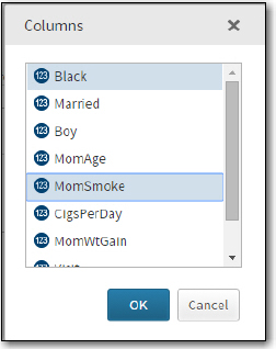
On the Data tab, select WORK.Birth_Wt_Sample (the name of your random sample), choose Weight (the weight values are in grams—1000 grams = 2.2 pounds) as the Dependent variable; choose Black (0 = not black, 1=black) and MomSmoke (0=no, 1=yes) as the factors. Select the factors in the usual way—holding down the control key and clicking your choices. See Figure 5:
Figure 5: How Factors are Selected
The next step is to click the Model tab to specify your model (Figure 6):
Figure 6: Selecting a Model
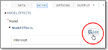
First, click Edit. This brings up the screen shown in Figure 7. Highlight the two variables Black and MomSmoke and click Full Factorial.
Figure 7: Select Black and MomSmoke in a Factorial Model

The factors in your model are then displayed on the right side of the screen (Figure 8):
Figure 8: The Task Displays Terms in Your Model

The two main effects are Black and MomSmoke, and the interaction term is shown as Black*MomSmoke.
Finally, click the Options tab to specify details for the ANOVA table and your selection of plots. In Figure 9, you see that Type 3 sums of squares is selected. Type 3 sums of squares shows the effect of each factor as if it were entered in the model last. Another way of saying this is that the analysis shows the effect of each factor after controlling for all the other factors.
Even though both main factors (Black and MomSmoke) have only two levels, you need to check the box labeled "Perform multiple comparisons" so that the program will compute the mean weights for each level of these factors.
Figure 9: Select Options

At the bottom of the Options screen, you can specify plot options (Figure 10). By choosing "Selected plots" from the plot menu, you can specify exactly what plots you want. For this example, options for an interaction plot and diagnostics plots were selected. You can choose to display the diagnostic plots as a panel (small plots all together on a single panel) or individual plots.
Figure 10: Select Plots

It's time to run the analysis. If you try this yourself, be aware that it can take several minutes to complete, depending on the speed of your computer and the memory allocated to your virtual computer.
You will see some output, but where are the plots? This brings up a very important lesson:
Before examining your results, take a moment to look at the SAS log to see if there are errors or warnings.
As you can see in Figure 11, the plots were suppressed because the number of points exceeded the default value of 5,000.
Figure 11: Check the SAS Log!

To fix the problem, go back to the Options tab and select No limit from the Maximum number of points to plot in the menu (Figure 12):
Figure 12: Adjust the Maximum Number of Points

Run the program again.
The first section of the output (Figure 13) shows class-level information. As we mentioned before, it is important to verify that the number of levels and the values for these factors are what you expect. The other piece of information that is often ignored, but is very important, is the number of observations read and used. In this example, these two numbers are the same, indicating that there are no missing values for the variables selected for this analysis.
Figure 13: Class-Level Information

Next, comes the ANOVA table.
Figure 14: The ANOVA Table

At the top, are the F and p-values for the model as a whole—below, you see the sum of squares, mean squares, F and p-values for each of the two factors and the interaction term. Both of the main factors are highly significant (Black and MomSmoke) and the interaction term is not significant (at the .05 level). Of course, you first need to examine the diagnostic plots to see if the ANOVA assumptions were satisfied.
Because the program produces so many diagnostic plots, only selected ones are included here. The first plot (Figure 15) shows the residuals (the difference between each data point and the predicted mean for each combination of the factors.
Figure 15: Inspecting the Residuals

From this plot, you can see that there are a few extra outliers on the low side and that the variance is similar in each of the four categories.
Figure 16 displays a histogram of the residuals. This looks symmetric and close enough to a normal distribution to satisfy this assumption.
Figure 16: Histogram of Residuals

Interpreting the Two-Way ANOVA Results
Now that you are satisfied that the ANOVA assumptions were correct, let's take a moment to look at the results. Both main effects (Black and MomSmoke) were significant as shown in the ANOVA table. Because the option to produce multiple comparisons was checked on the Options tab, you obtain the following two tables:
First, you see the LSMEANS for the variable Black (Figure 17):
Figure 17: LSMEANS for Black

The means shown in this table are means computed from the linear model. If there are no missing values in your data set (as is the case in this data set), these means are exactly the same means that you would compute by adding up all the weights for babies born from black or non-black mothers and dividing by the number of mothers in each group, respectively. If there are missing values for any of the observations, the LSMEANS will produce a slightly different value. You see that babies born from black mothers are lighter than babies born from non-black mothers (the difference is about 236 grams (about half a pound)). The output also shows this difference along with the 95% confidence limits. Notice that these limits do not include 0, as you expect because the difference is significant at the .05 level.
The same information is displayed in Figure 18, for the variable MomSmoke.
Figure 18: LSMEANS for MomSmoke

Babies born to mothers who smoke are approximately 263 grams (about half a pound) lighter than babies born to mothers who do not smoke.
Interpreting Models with Significant Interactions
It is important to inspect the interaction term before you interpret main effects in a factorial model. You can use the same data set (Birth_Wt_Sample) used in the previous example to demonstrate a model with a significant interaction term.
If you run a factorial model with MomSmoke and Married as the two factors, you obtain the following:
Figure 19: Notice a Significant Interaction Term

You see significant effects for the two factors as well as the interaction term. Because this analysis was run with the option to produce multiple comparisons, you can see the means for each combination of the two factors (Figure 20).
Figure 20: Adjusted Cell Means

It is easier to see this graphically (see Figure 21):
Figure 21: Interaction Plot

(Note: The lines between the pairs of means on this plot were added by the author; they are not included in the output.) On the x-axis, you see each combination of the two factors. The highest birth weights are found for babies whose moms do not smoke and who are married; the lowest birth weights are found for babies whose moms smoke and who are not married. However, the effect of smoking or not smoking is different for married versus unmarried moms. If there were no interactions between these factors, the two lines on the plot would be parallel. The different slopes of the two lines (and the significant p-value for the interaction term) indicate that the two factors interact with each other.
Conclusions
This chapter has demonstrated simple two-way models. Much more complex models with nested and/or crossed factors can be analyzed with the N-Way ANOVA task. Analysis of the birth weight data used in this chapter may be more meaningful by regression techniques or, if the birth weights were grouped, logistic regression. Those topics are discussed in later chapters of this book. One other thing: If you are pregnant, don't smoke!
Problems
9-1: Using the Blood_Pressure.xlsx workbook, create a temporary SAS data set (call it BP). Run a two-way ANOVA model with DBP as the dependent variable with Drug and Gender as factors. Run a full factorial model. Be sure to check the interaction term before interpreting the main effects. Include diagnostic plots in your output. Using the Tukey method, determine which Drug groups are different (if there are any).
9-2: Using the SASHELP data set HEART, run a two-way ANOVA using Weight as the dependent variable and Sex and Chol_Status (cholesterol status) as factors. Request multiple comparisons for main effects and Type 3 sum of squares only. Suppress all plots. What comparisons, if any, are significant for Chol_Status?
9-3: Using the workbook Diabetes.xls, create a temporary SAS data set (call it Diabetes) and perform a two-way ANOVA with Glucose as the dependent variable and Insulin and Diet_Drinks as factors (independent) variables. Be sure to check whether the interaction term is significant before exploring the main effects. Request multiple comparison for all effects as well as an interaction plot.
9-4: Rerun problem 9-3 except use a filter to omit the group Diet_Drinks = 'Sometimes'. Your filter statement should be:
Diet_Drinks ne 'Sometimes'
Examine the Tukey multiple comparisons for all significant factors.
9-5: You have measured the left ventricular ejection fraction (LVEF) on three groups of subjects with congestive heart failure (CHF). LVEF is the percent that the left ventricle contracts compared to a normal heart. The three groups represent 1) Placebo, 2) Calcium channel blocker, and 3) Lasix. In addition, each subject is in a normal weight group or an overweight group. The experiment resulted in the following:
Group Weight Data values for LVEF
-------------------------------------------
Placebo Overweight 55 57 57 40 52
Placebo Norm: 58 80 55 48 62
Calcium Overweight 57 78 84 72 78
Calcium Normal 65 80 81 57 55
Lasix Overweight 60 65 48 64 40
Lasix Normal 70 62 60 57 67
Run the SAS program below to create the CHF data set. The variables in this data set are Subj, Group (Placebo, Calcium, or Lasix), Weight, and LVEF.
data CHF;
do Group = 'Placebo','Calcium','Lasix';
do Weight = 'Overweight','Normal';
do Subj = 1 to 5;
input LVEF @@;
output;
end;
end;
end;
datalines;
55 57 57 40 52
58 80 55 48 62
57 78 84 72 78
65 80 81 57 55
60 65 48 64 40
70 62 60 57 67
;
You can see an explanation of how this program works from problem 8-6. The only difference is the addition of one more DO loop that creates the weight group variable.
Run a two-way ANOVA testing each of the main effects: Group and Weight.