
In data mining, we use ensemble methods, which means using multiple learning algorithms to obtain better predictive results than applying any single learning algorithm on any statistical problem. This section will provide an overview of popular ensemble methods such as bagging, boosting, and random forests
Bagging is also known as Bootstrap aggregating. It is designed to improve the stability and accuracy of machine-learning algorithms. It helps avoid over fitting and reduces variance. This is mostly used with decision trees.
Bagging involves randomly generating Bootstrap samples from the dataset and trains the models individually. Predictions are then made by aggregating or averaging all the response variables:
- For example, consider a dataset (Xi, Yi), where i=1 …n, contains n data points.
- Now, randomly select B samples with replacements from the original dataset using Bootstrap technique.
- Next, train the B samples with regression/classification models independently. Then, predictions are made on the test set by averaging the responses from all the B models generated in the case of regression. Alternatively, the most often occurring class among B samples is generated in the case of classification.
Random forests are improvised supervised algorithms than bootstrap aggregation or bagging methods, though they are built on a similar approach. Unlike selecting all the variables in all the B samples generated using the Bootstrap technique in bagging, we select only a few predictor variables randomly from the total variables for each of the B samples. Then, these samples are trained with the models. Predictions are made by averaging the result of each model. The number of predictors in each sample is decided using the formula m = √p, where p is the total variable count in the original dataset.
Here are some key notes:
- This approach removes the condition of dependency of strong predictors in the dataset as we intentionally select fewer variables than all the variables for every iteration
- This approach also de-correlates variables, resulting in less variability in the model and, hence, more reliability
Refer to the R implementation of random forests on the iris dataset using the randomForest package available from CRAN:
#randomForest
library(randomForest)
data(iris)
sample = iris[sample(nrow(iris)),]
train = sample[1:105,]
test = sample[106:150,]
model =randomForest(Species~.,data=train,mtry=2,importance =TRUE,proximity=TRUE)
model
Call:
 randomForest(formula = Species ~ ., data = train, mtry = 2, importance = TRUE,      proximity = TRUE)
               Type of random forest: classification
                     Number of trees: 500
No. of variables tried at each split: 2

        OOB estimate of  error rate: 5.71%
Confusion matrix:
           setosa versicolor virginica class.error
setosa         40          0         0  0.00000000
versicolor      0         28         3  0.09677419
virginica       0          3        31  0.08823529

pred = predict(model,newdata=test[,-5])
pred
pred
       119         77         88         90         51         20         96
 virginica versicolor versicolor versicolor versicolor     setosa versicolor
         1          3        118        127          6        102          5
    setosa     setosa  virginica  virginica     setosa  virginica     setosa
        91          8         23        133         17         78         52
versicolor     setosa     setosa  virginica     setosa  virginica versicolor
        63         82         84        116         70         50        129
versicolor versicolor  virginica  virginica versicolor     setosa  virginica
       150         34          9        120         41         26        121
 virginica     setosa     setosa  virginica     setosa     setosa  virginica
       145        138         94          4        104         81        122
 virginica  virginica versicolor     setosa  virginica versicolor  virginica
        18        105        100
    setosa  virginica versicolor
Levels: setosa versicolor virginicaUnlike with bagging, where multiple copies of Bootstrap samples are created, a new model is fitted for each copy of the dataset, and all the individual models are combined to create a single predictive model, each new model is built using information from previously built models. Boosting can be understood as an iterative method involving two steps:
- A new model is built on the residuals of previous models instead of the response variable
- Now, the residuals are calculated from this model and updated to the residuals used in the previous step
The preceding two steps are repeated for multiple iterations, allowing each new model to learn from its previous mistakes, thereby improving the model accuracy:
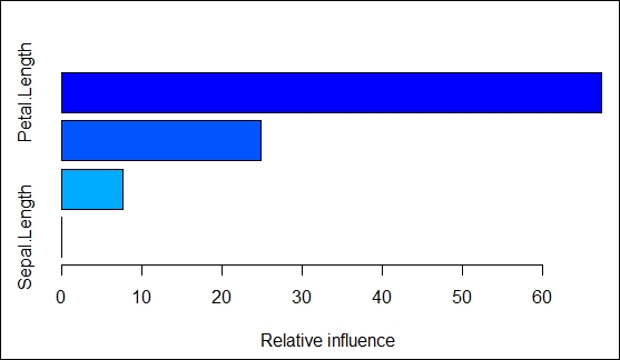
#Boosting in R
library(gbm)
data(iris)
sample = iris[sample(nrow(iris)),]
train = sample[1:105,]
test = sample[106:150,]
model = gbm(Species~.,data=train,distribution="multinomial",n.trees=5000,interaction.depth=4)
summary(model)
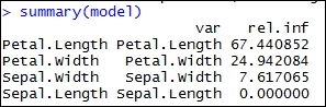
The output of the preceding code is as follows:
In the following code snippet, the output value for the predict() function is used in the apply() function to pick the response with the highest probability among each row in the pred matrix. The resultant output from the apply() function is the prediction for the response variable:
//the preceding summary states the relative importance of the variables of the model.

pred = predict(model,newdata=test[,-5],n.trees=5000)

pred[1:5,,]
        setosa versicolor virginica
[1,]  5.630363  -2.947531 -5.172975
[2,]  5.640313  -3.533578 -5.103582
[3,] -5.249303   3.742753 -3.374590
[4,] -5.271020   4.047366 -3.770332
[5,] -5.249324   3.819050 -3.439450

//pick the response with the highest probability from the resulting pred matrix, by doing apply(.., 1, which.max) on the vector output from prediction.
p.pred <- apply(pred,1,which.max)
p.pred
[1] 1 1 3 3 2 2 3 1 3 1 3 2 2 1 2 3 2 2 3 3 1 1 3 1 3 3 3 1 1 2 2 2 2 2 2 2 1 1 3 1 2
[42] 1 3 2 3