The R command to build the model is the same as the previous chapter. Now, the technique is called UBCF:

recommender_models <- recommenderRegistry$get_entries(dataType = "realRatingMatrix")
recommender_models$UBCF_realRatingMatrix$parameters

Some relevant parameters are:

Let's build a recommender model leaving the parameters to their defaults:

recc_model <- Recommender(data = recc_data_train, method = "UBCF")recc_model
## Recommender of type 'UBCF' for 'realRatingMatrix' ## learned using 451 users.

Let's extract some details about the model using getModel:

model_details <- getModel(recc_model)

Let's take a look at the components of the model:

names(model_details)

Apart from the description and parameters of model, model_details contains a data slot:

model_details$data
## 451 x 332 rating matrix of class 'realRatingMatrix' with 43846 ratings.
## Normalized using center on rows.

The model_details$data object contains the rating matrix. The reason is that UBCF is a lazy-learning technique, which means that it needs to access all the data to perform a prediction.

In the same way as the IBCF, we can determine the top six recommendations for each new user:

n_recommended <- 6
recc_predicted <- predict(object = recc_model, newdata = recc_data_test, n = n_recommended) recc_predicted
## Recommendations as 'topNList' with n = 6 for 109 users.

We can define a matrix with the recommendations to the test set users:

recc_matrix <- sapply(recc_predicted@items, function(x){colnames(ratings_movies)[x]
})
dim(recc_matrix)
## [1]   6 109

Let's take a look at the first four users:

recc_matrix[, 1:4]

We can also compute how many times each movie got recommended and build the related frequency histogram:

number_of_items <- factor(table(recc_matrix))
chart_title <- "Distribution of the number of items for UBCF"

Let's build the distribution chart:

qplot(number_of_items) + ggtitle(chart_title)

The following image displays the distribution of the numbers of items for UBCF:

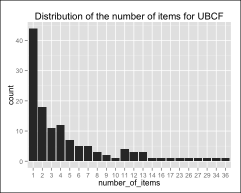
Compared with the IBCF, the distribution has a longer tail. This means that there are some movies that are recommended much more often than the others. The maximum is 29, compared with 11 for IBCF.

Let's take a look at the top titles:

number_of_items_sorted <- sort(number_of_items, decreasing = TRUE)
number_of_items_top <- head(number_of_items_sorted, n = 4)
table_top <- data.frame(names(number_of_items_top), number_of_items_top)
table_top

The preceding table is continued as follows:

Comparing the results of UBCF with IBCF helps in understanding the algorithm better. UBCF needs to access the initial data, so it is a lazy-learning model. Since it needs to keep the entire database in memory, it doesn't work well in the presence of a big rating matrix. Also, building the similarity matrix requires a lot of computing power and time.

However, UBCF's accuracy is proven to be slightly more accurate than IBCF, so it's a good option if the dataset is not too big.

In the previous two sections, we built recommendation models based on user preferences, since the data displayed the rating for each purchase. However, this information is not always available. The following two scenarios can take place:

In these contexts, we can build a user-item matrix whose values would be 1 if the user purchased (or liked) the item, and 0 otherwise. This case is different from the previous cases, so it should be treated separately. Similar to the other cases, the techniques are item-based and user-based.

In our case, starting from ratings_movies, we can build a ratings_movies_watched matrix whose values will be 1 if the user viewed the movie, and 0 otherwise. We built it in one of the Binarizing the data sections.

We can build ratings_movies_watched using the binarize method:

ratings_movies_watched <- binarize(ratings_movies, minRating = 1)

Let's take a quick look at the data. How many movies (out of 332) did each user watch? Let's build the distribution chart:

qplot(rowSums(ratings_movies_watched)) + stat_bin(binwidth = 10) + geom_vline(xintercept = mean(rowSums(ratings_movies_watched)), col = "red", linetype = "dashed") + ggtitle("Distribution of movies by user")

The following image shows a distribution of movies by user:

On the average, each user watched about 100 movies, and only a few watched more than 200 movies.

In order to build a recommendation model, let's define a training set and a test set:

which_train <- sample(x = c(TRUE, FALSE), size = nrow(ratings_movies), replace = TRUE, prob = c(0.8, 0.2))
recc_data_train <- ratings_movies[which_train, ]
recc_data_test <- ratings_movies[!which_train, ]

We are now ready to build the IBCF and UBCF models.

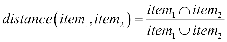
The first step with IBCF is defining a similarity between items. In the case of binary data, distances such as the correlation and the cosine don't work properly. A good alternative is the Jaccard index. Given two items, the index is computed as the number of users purchasing both the items divided by the number of users purchasing at least one of them. Let's start from and , which are the sets of users purchasing the first and second item, respectively. The "∩" symbol refers to the intersection of two sets, that is, the items contained in both. The "U" symbol refers to the union of two sets, that is, the items contained in at least one of them. The Jaccard index is the number of elements in the intersection between the two sets, divided by the number of elements in their union.

We can build the IBCF filtering model using the same commands as in the previous chapters. The only difference is the input parameter method equal to Jaccard:

recc_model <- Recommender(data = recc_data_train, method = "IBCF", parameter = list(method = "Jaccard"))
model_details <- getModel(recc_model)

Like in the previous sections, we can recommend six items to each of the users in the test set:

n_recommended <- 6
recc_predicted <- predict(object = recc_model, newdata = recc_data_test, n = n_recommended)
recc_matrix <- sapply(recc_predicted@items, function(x){colnames(ratings_movies)[x]
})

Let's see the recommendations for the first four users.

recc_matrix[, 1:4]

The approach is similar to IBCF using a rating matrix. Since we are not taking account of the ratings, the result will be less accurate.